Vol. 9 (2020), No. 1, 85 - 94
CURVATURE IN HILBERT GEOMETRIES
ÁRPÁD KURUSA
Abstract. We provide more transparent proofs for the facts that the curvature of a Hilbert geometry in the sense of Busemann can not be non-negative and a point of non-positive curvature is a projective center of the Hilbert geometry. Then we prove that the Hilbert geometry has non-positive curvature at its projective centers, and that a Hilbert geom- etry is a Cayley–Klein model of Bolyai’s hyperbolic geometry if and only if it has non-positive curvature at every point of its intersection with a hyperplane. Moreover a 2-dimensional Hilbert geometry is a Cayley–
Klein model of Bolyai’s hyperbolic geometry if and only if it has two points of non-positive curvature and its boundary is twice differentiable where it is intersected by the line joining those points of non-positive curvature.
1. Introduction
A Hilbert geometry is a pair (I, dI) of an open, strictly convex domain I ⊂Rn, and theHilbert metric [2, page 297]dI:I × I →Rgiven by (1.1) dI(X, Y) =
(
0, if X=Y ,
1 2
ln(A, B;X, Y)
, if X6=Y, whereAB=I ∩XY . Every geodesic `˜of a Hilbert geometry (I, dI) is the intersection I ∩` ofI with a straight line `.
Busemann posed the problem [3, 34th on p. 406] if a Hilbert geometry that has non-positive curvature at every point is a Cayley–Klein model of Bolyai’s hyperbolic geometry. This was affirmatively answered in [4, The- orem, p. 119], where Kelly and Strauss showed that if a point in a Hilbert geometry(I, dI) has non-positive curvature then it is a projective center of I. They finished [4] by a conjecture that a Hilbert geometry can contain no points of non-negative curvature. This was proved in [6], where Kelly and Strauss closed the paper by discussing the problem if
(1.2) a projective center has non-positive curvature.
In this paper we provide a bit more transparent proofs for the above men- tioned results of Kelly and Strauss, and then we prove (1.2) in Theorem4.2.
Finally we obtain sharper affirmative answers for Busemann’s problem [3, 34th on p. 406] in Section5 as easy consequences.
Research was supported by NFSR of Hungary (NKFIH) under grant numbers K 116451 and KH_18 129630, and by the Ministry of Human Capacities, Hungary grant 20391- 3/2018/FEKUSTRAT..
Keywords and phrases: Hilbert metric, Busemann curvature, projective center (2020) Mathematics Subject Classification: 53A35, 53A20; 52A20
Received: 31.01.2020. In revised form: 20.03.2020. Accepted: 13.02.2020.
85
2. Notations and preliminaries
Points of Rn are denoted as A, B, . . .. The open segment with endpoints A and B is denoted by AB, and AB denotes the line throughA andB.
We denote theaffine ratio of the collinear pointsA, B andC by(A, B;C) that satisfies (A, B;C)−−→
BC = −→
AC. The affine cross ratio of the collinear points A, B andC, D is(A, B;C, D) = (A, B;C)/(A, B;D) [2, page 243].
In this article I is an open, strictly convex domain in Rn, where n≥ 2.
We shall use without further notice the well-known fact [8, Theorem 25.3], that a convex function has both one-sided derivative at every point, and its derivative is strictly monotone, hence it is differentiable everywhere except at most a countable set. Moreover, a convex function has a second-order quadratic expansion at almost every point of its domain by Alexandrov’s theorem [1] (see [9, Theorem 2.1]). These are called Alexandrov points, and in the expansions the usual big-O notation is used.
Given a point P ∈ I, the polar P∗ of P is defined as the locus of every pointXthat is the harmonic conjugate ofP with respect toAandB, where AB = I ∩P X. It is easy to see [7, p. 64] that the polar P∗ of a point P ∈ I ⊂Rn is a hyperplane outside I if and only ifP is aprojective center ofI, i.e. there is a projectivity$such that$(P)is the affine center of$(I).
It is well known that a Hilbert geometry is the Cayley–Klein model of Bolyai’s hyperbolic geometry if and only if it is given by an ellipsoid [2, 29.3].
A Hilbert geometry at a point O haspositive, non-negative,non-positive and negative curvature in the sense of Busemann if there exists a neighbor- hood U of O such that for every pair of points P, Q∈ U we have
2dI( ˆP ,Q)ˆ > dI(P, Q), 2dI( ˆP ,Q)ˆ ≥dI(P, Q), 2dI( ˆP ,Q)ˆ ≤dI(P, Q), 2dI( ˆP ,Q)ˆ < dI(P, Q),
respectively, whereP ,ˆ Qˆ are the respectivedI-midpoints of the geodesic seg- ments OP and OQ [3, (36.1) on p. 237]. If neither of the cases is satisfied in any neighborhood of O, then we say that the curvature is indeterminate [4, Definition 1]4. A projectivity $is clearly a bijective isometry of (I, dI) to ($(I), d$(I)), hence
(2.1) Busemann’s curvature is a projective invariant.
3. Preparations
We consider a Hilbert geometry(I, dI) and a point O inI.
Lemma 3.1 ([4, Lemma 1 and Corollary]). There exist two (maybe ideal) points X and Y in O∗ such that line XY does not intersect I, and ∂I is differentiable at the points in ∂I ∩(OX∪OY).
Proof. There is at least one chord AB of I which is bisected by O. Then the harmonic conjugate X¯ of O with respect to A and B is on the line at infinity.
4Notice that positivity or negativity of the curvature in [4, Definition 1] corresponds to non-negativity, respectively non-positivity in our terms.
If X¯ is the only point of O∗ at infinity, then O∗ cannot completely lie within the strip formed by the two supporting lines of I which are parallel to AB, because otherwise, as O∗ is a connected curve, it would intersect I.
Thus, a further point Y¯ ofO∗ outside this strip exists.
If X¯ is not the only point ofO∗ at infinity, then let that point be Y¯. Then line X¯Y¯ does not intersect I, but intersects O∗ in the points X¯ and Y¯.
Since all but a denumerable set of points of∂I are points of differentiabil- ity, we may choose points X ∈O∗ and Y ∈O∗ near X¯ and Y¯, respectively, so that ∂I is differentiable at the points in∂I ∩(OX∪OY), and XY does
not intersect I.
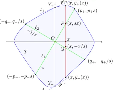
Let `1 and `2 be straight lines through O, and let l± be straight lines through O such that
(3.1) −(`1, `2;l−, l+)≥1.
Denote by Y± the points wherel+ intersects∂I so that
(3.2) (Y−, Y+;O)2 ≤1.
Let t± be the tangent lines of∂I at Y±.
Fix a coordinate system so that O = (0,0), l− is the x-axis, l+ is the y-axis, and Y+ is in the upper half-plane. Forx in a small neighborhood of 0, let y± be the continuous functions of x such that (x, y±(x)) are the two points of ∂I with abscissa x, and Y±= (0, y±(0)) so±y±(x)>0.
Fix an Euclidean metric d such that the two axes and the lines `1 and
`2 are perpendicular to each other, respectively. Let s > 0 be the slope of
`1, hence the slope of `2 is −1/s. Let m± be the slope of t±, and if the intersection of t± and thex-axis exists, then denote it byT±. So Figure 3.1 shows what we have.
I
O Y+
Y−
(p+, p+s)
(−p−,−p−s) (−q−, q−/s)
(q+,−q+/s)
`1
s
`2
−1/s t+
m+
t−
m− x P (x, sx)
Q (x,−x/s) (x, y+(x))
(x, y−(x))
Figure 3.1. The configuration in euclidean plane.
Let p±, q± > 0 be such that (±p±,±p±s) are the points of `1 ∩∂I, and (±q±,∓q±/s) are the points of `2∩∂I.
Lemma 3.2. If O is the affine midpoint of the chords`1∩ I and`2∩ I, and the points Y± are Alexandrov points of ∂I, then in a small neighborhood of O we have
(3.3) dI(P, Q)−2dI( ˆP ,Q)ˆ ≥ x2 2s
s2m−
y2−(0) − m+ y2+(0)
+x3O(1),
where P ,ˆ Qˆ are the dI-midpoints of the geodesic segments OP and OQ, re- spectively.
Proof. Since O is the midpoint of the chords `˜1 = `1∩ I and `˜2 =`2∩ I, we have p:=p+=p− and q :=q+=q−.
We have to show that there is anε >0such that the pointsP = (x, sx)∈
`˜1,Q= (x,−x/s)∈`˜2 (x∈(0, ε)), and the respectivedI-midpointsP ,ˆ Qˆ of the geodesic segments OP andOQ satisfy (3.3).
The strict triangle inequalitydI( ˆP ,Q)ˆ < dI( ˆP ,P¯) +dI( ¯P ,Q) +¯ dI( ¯Q,Q),ˆ whereP¯ = (x2,sx2) andQ¯ = (x2,−x2s), gives
dI(P, Q)−2dI( ˆP ,Q)ˆ
≥(dI(P, Q)−2dI( ¯P ,Q))¯ −2(dI( ˆP ,P¯) +dI( ¯Q,Q)),ˆ (3.4)
so it is enough to estimate the right-hand side of this inequality from below.
By (1.1) and the Taylor series expansion of the logarithm, we have dI(O, P) = 1
2lnp+x p−x = 1
2
ln 1 +x
p
−ln 1−x
p
= 1 2
∞
X
i=1
1−(−1)i i
x p
i
,
hence dI(O, P) =
∞
X
j=0
1 2j+ 1
x p
2j+1
, and dI(O,P) =¯
∞
X
j=0
2−1−2j 2j+ 1
x p
2j+1
.
The same calculation for Qand Q¯ leads to dI(O, Q) =
∞
X
j=0
1 2j+ 1
x q
2j+1
, and dI(O,Q) =¯
∞
X
j=0
2−1−2j 2j+ 1
x q
2j+1
.
Further, as dI(O,P) =ˆ dI(O, P)/2, and dI(O,Q) =ˆ dI(O, Q)/2, the above formulas also imply
dI( ¯P ,Pˆ) =|dI(O,Pˆ)−dI(O,P¯)|= 1 2
∞
X
j=1
1−2−2j 2j+ 1
x p
2j+1
, (3.5)
dI( ¯Q,Q) =ˆ |dI(O,Q)ˆ −dI(O,Q)|¯ = 1 2
∞
X
j=1
1−2−2j 2j+ 1
x q
2j+1
. (3.6)
Since dI(P, Q) = 12
lnsx−y
−(x)
y+(x)−sx : −x/s−yy −(x)
+(x)+x/s
by (1.1), the Taylor series expansion of the logarithm gives
dI(P, Q) = 1 2
ln
1 + sx
−y−(x)
−ln
1− sx y+(x)
+ + ln
1 + x/s y+(x)
−ln
1− x/s
−y−(x)
= 1 2
X∞
i=1
1−(−1)i i
sx
−y−(x) i
+
∞
X
i=1
1−(−1)i i
x/s y+(x)
i
=
∞
X
j=0
−s2j+1 2j+ 1
x y−(x)
2j+1
+
∞
X
j=0
s−2j−1 2j+ 1
x y+(x)
2j+1
. (3.7)
In the same way dI( ¯P ,Q) =¯ 12
lnsx/2−y
−(x/2)
y+(x/2)−sx/2 :−x/2/s−yy −(x/2)
+(x/2)+x/2/s
implies dI( ¯P ,Q) =¯
∞
X
j=0
−s2j+1 2j+ 1
x/2 y−(x/2)
2j+1
+
∞
X
j=0
s−2j−1 2j+ 1
x/2 y+(x/2)
2j+1
(3.8) .
Since the pointsY±are Alexandrov points of∂I, we have the Taylor series expansions y¯±(t) = ¯y±(0) +t¯y±0 (0) +t2O(1) of the functions y¯± := 1/y±. For easy handling of this we define y¯±hii(0) (i = 0,1,2) so that y¯±(t) = P2
i=0tiy¯hii±(0)/i!.
Substituting (3.5), (3.6), (3.7), (3.8), and the above Taylor expansion of
¯
y±(x) into the right-hand side of (3.4), we obtain (dI(P, Q)−2dI( ¯P ,Q))¯ −2(dI( ˆP ,P¯) +dI( ¯Q,Q))ˆ
=
∞
X
j=0
−s2j+1 2j+ 1
X2
i=0
xi+1y¯−hii(0) i!
2j+1
+
∞
X
j=0
s−2j−1 2j+ 1
X2
i=0
xi+1y¯+hii(0) i!
2j+1
−
−2
∞
X
j=0
−s2j+1 2j+ 1
X2
i=0
xi+1y¯−hii(0) i!2i+1
2j+1
−2
∞
X
j=0
s−2j−1 2j+ 1
X2
i=0
xi+1y¯hii+(0) i!2i+1
2j+1
−
−
∞
X
j=1
1−2−2j 2j+ 1
x p
2j+1
−
∞
X
j=1
1−2−2j 2j+ 1
x q
2j+1
.
Separating the summands with index j = 0 from the sums with running variablej, and moving them to the beginning result in
(dI(P, Q)−2dI( ¯P ,Q))¯ −2(dI( ˆP ,P) +¯ dI( ¯Q,Q))ˆ
=−s
2
X
i=0
xi+1y¯−hii(0) i! +1
s
2
X
i=0
xi+1y¯hii+(0) i! +s
2
X
i=0
xi+1y¯−hii(0) i!2i −
−1 s
2
X
i=0
xi+1y¯hii+(0)
i!2i +x3O(1).
The summands with indexi= 0just cancel each other, the summands with index i= 2 has multiplier x3, so we obtain
(dI(P, Q)−2dI( ¯P ,Q))¯ −2(dI( ˆP ,P¯) +dI( ¯Q,Q))ˆ
=x2 1
2sy¯+0 (0)−s
2y¯0−(0)
+x3O(1).
Since y±:= 1/¯y±, one gets e:= 1
2sy¯0+(0)−s
2y¯−0 (0) = −1 2s
y0+(0) y2+(0)+s
2 y0−(0) y2−(0) = 1
2s
s2m−
y−2(0)− m+ y+2(0)
that proves the lemma.
4. Curvature in Hilbert geometry
Firstly we reprove the result of [6] using our preparatory Lemma 3.2.
Theorem 4.1. A Hilbert geometry can not have positive or non-negative curvature at any point.
Proof. It is enough to prove that
(4.1)
through every point O of a Hilbert geometry (I, dI) there are two geodesics`˜1 and`˜2 such that in any suitable small open neighborhood U of O inequality 2dI( ˆP ,Q)ˆ < dI(P, Q) is fulfilled for some points P ∈`˜1∩ U andQ∈`˜2∩ U, whereP ,ˆ Qˆ ∈ U are the dI-midpoints of the geodesic segments OP and OQ, respectively.
As two geodesics lie always in a common plane, it is enough to prove (4.1) in the plane. Let O be an arbitrary point inI ⊂R2.
By Lemma3.1, there is a projectivity$such that$(O)is the affine center of at least two geodesics $(˜`1) and $(˜`2). So taking (2.1) into account, we assume from now on that O is the affine center of the segments `1∩ I and
`2∩ I.
Choose the straight linesl±throughO so thatY±are Alexander points of
∂I, and −(`1, `2;l−, l+) >1. This is possible because if equality happened in (3.1), then rotatingl− a little bit helps. So by (3.2) we have
(4.2) −(`1, `2;l−, l+)>(Y−, Y+;O)2.
If either one of the tangentst±is parallel tol−, then slightly rotatel−around O so that it keeps the properties required above and intersects the tangents t± in some points, say T± =t±∩l−. If |(T+, T−;O)|< |(Y+, Y−;O)|, then change the indexing from ±to ∓, so we have|(T+, T−;O)| ≥ |(Y+, Y−;O)|.
Now we choose a coordinate system so that the positive half of thex-axis contains T−. Figure 4.1shows what we have if O∈T−T+.
O Y+
Y−
I
l+
`1
`2
T+ T−
t+
t−
l−
Figure 4.1. The affine configuration ifO∈ I ∩T+T−.
By Lemma 3.2 statement (4.1) fulfills if m−
2sy2+(0) s2y
2 +(0) y−2(0) −mm+
−
, the main term in (3.3), is positive, i.e. s2y
2 +(0)
y2−(0) > mm+−. Observe that (4.2) implies s2y+2(0)
y−2(0)=−−s 1/s
|Y+O|2
|OY−|2=−(`1, `2;l−)
(Y−, Y+;O)2=−(`1, `2;l−, l+) (Y−, Y+;O)2 >1.
So we need to prove that mm+
− ≤ 1. If 0 < (T+, T−;O), then m+ < 0 and therefore mm+
− <0. If(T+, T−;O)<0, then m+
m−
= |Y+O|/|T+O|
|OY−|/|OT−| = |Y+O|
|OY−|
|OT−|
|T+O| = |(Y+, Y−;O)|
|(T+, T−;O)| ≤1,
so the proof is complete.
We use again Lemma 3.2to improve [4, the first statement of Theorem].
Theorem 4.2. A point O in the Hilbert geometry (I, dI) has non-positive curvature if and only if it is a projective center of I.
Proof. Firstly we prove the necessity part5.
We assume that (I, dI) has non-positive curvature at O, and have to prove that O∗ is a hyperplane. For this it is enough to prove that every plane section of O∗ is a straight line. So, from now on we assume that I ⊂R2, and need to prove that
there is a projectivity $ such that $(O) is the affine center of $(I).
By Lemma3.1, there is a projectivity$such that$(O)is the affine center of at least two geodesics $(˜`1) and $(˜`2), so, according to (2.1), we may assume without loss of generality that O is the affine center of the segments
`1∩ I and `2∩ I.
This time we choose the straight lines l± throughO so that (4.3) −(`1, `2;l−, l+) = 1,
Y± are Alexander points of ∂I, and l− intersects both t±. This can be achieved easily, because except the two directions, where l− is parallel to one of the tangents t±, and where a point Y± is not an Alexander point of
∂I, the direction of l− can be chosen freely, and l+ is determined change accordingly by (4.3).
Choose the direction of thex-axes so that the abscissa ofT− be positive.
Again Figure 4.1shows what we have if O ∈T+T−.
Since the Busemann curvature is non-positive, i.e. 2dI( ˆP ,Q)ˆ ≥dI(P, Q), the main term in (3.3) of Lemma 3.2 should vanish, i.e. s2m−
y2−(0) = ym2+ +(0). However s2=−1/s−s=−(`1, `2;l−) =−(`1, `2;l−, l+) = 1, so−y
0
−(0±) y−2(0) = y
0 +(0±) y+2(0)
follows, where the sign±at0±is determined by the direction of thex-axis.
Rearrangement gives
y+(0) y+(0)
y+0 (0±) = (−y−)(0) (−y−)(0) (−y−)0(0±),
5This is [4, first statement of Theorem]
that, as ±y+(0) =d(O, Y±) and ±y±(0)/(±y0±(0)) = d(O, T±), means that the triangles 4OY+T+ and4OY−T− have equal areas.
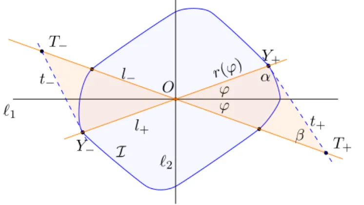
Change now to a Euclidean metricde such that`1 and `2 are orthogonal.
Let the direction vector of l+ be(cosϕ,sinϕ), hence the direction vector of l− is (cosϕ,−sinϕ), and let r be the radial function of ∂I from the point O, hence Y+ =r(ϕ)(cosϕ,sinϕ)andY−=r(ϕ+π)(cos(ϕ+π),sin(ϕ+π)).
See Figure 4.2.
O
Y+
Y− I
`2
`1
ϕ ϕ l−
T−
T+
l+
r(ϕ)
t+
t− α
β
Figure 4.2. We havearea(4OY+T+) = area(4OY−T−)for everyϕ.
Define α :=∠(O, Y+, T+), β :=π−α−2ϕ. Thencotα =−r(ϕ)/r(ϕ)˙ and a(ϕ) := 2 area(4OY+T+) =r2(ϕ)sin(2ϕ)sinβ sinα, hence
sin(2ϕ)
a(ϕ) =r−2(ϕ)sin(2ϕ+α)
sinα =r−2(ϕ) sin(2ϕ) cotα+ cos(2ϕ)
= sin(2ϕ)−r(ϕ)˙
r3(ϕ) + cos(2ϕ) 1 r2(ϕ) = 1
2
sin(2ϕ) r2(ϕ)
0
.
Thus, we have sin(2ϕ)
r2(ϕ) 0
= sin(2ϕ)
a(ϕ) = sin(2(ϕ+π)) a(ϕ+π) =
sin(2(ϕ+π)) r2(ϕ+π)
0
,
and also limϕ→0 sin(2ϕ)
r2(ϕ) = 0 = limϕ→0 sin(2(ϕ+π))
r2(2(ϕ+π)). Thus r(ϕ) ≡ r(ϕ+π) follows, meaning that I is affine symmetric with respect to O.
Thus the necessity part of the theorem is proved.
Next we prove the sufficiency part6.
We assume that O is a projective center of I, and we have to prove that
(4.4)
there is a suitable small open neighborhood U of O that for every geodesics `˜1 and `˜2 through O inequality 2dI( ˆP ,Q)ˆ ≤ dI(P, Q) is fulfilled for every points P ∈ `˜1 ∩ U and Q ∈ `˜2 ∩ U, where P ,ˆ Qˆ ∈ U are the dI-midpoints of the geodesic segments OP and OQ, respectively.
According to (2.1), we may assume without loss of generality thatO is the affine center ofI. Since two geodesics lie in a common plane, it is enough to prove (4.4) in the plane, so we assume thatO is the affine center ofI ⊂R2. Choose the straight linesl± so that Y± are Alexander points of∂I, and (4.5) −(`1, `2;l−, l+)>1.
6The last paragraph of [6] argues that this “does not seem easy”.
This is possible because if equality happened in (3.1), then rotating l− a little bit helps. Moreover, if t+is parallel to l−, then one can slightly rotate l− around O so that (4.5) remains valid and intersects t+. Thus, we can assume that the point T+ exists. Since O is the affine center ofI, we have t+ kt−, so also pointT− exists, and O is clearly the affine center of T−T+.
Now we fix the coordinate system and euclidean metric given in Section3 so that the positive half of the x-axes contains T−. Again Figure 4.1shows what we have.
By Lemma 3.2statement (4.4) fulfills if the main term m−
2sy2+(0) s2y
2 +(0) y−2(0) −
m+
m−
in (3.3) is positive. This fulfills because mm+
−= 1 by t+ k t−, m− > 0, and s2y
2 +(0)
y2−(0) −1 =−1/s−s −1 =−(`1, `2;l−, l+)−1>0 by (4.5).
5. Consequences
The following statements sharpen and extend the solution [4, second state- ment in Theorem] of Kelly and Strauss given to Busemann’s [3, Problem 34, p. 406].
Theorem 5.1. A Hilbert geometry is a Cayley–Klein model of Bolyai’s hy- perbolic geometry if and only if there is a hyperplane intersecting the Hilbert geometry so that every point of the intersection is of non-positive curvature.
Proof. If the Hilbert geometry is a Cayley–Klein model of Bolyai’s hyper- bolic geometry, then it has non-positive curvature at every point.
If there is a hyperplane intersecting the Hilbert geometry so that the Hilbert geometry has non-positive curvature at every point in the inter- section, then all these points are projective centers by Theorem 4.2, and therefore [7, Theorem 3.3(a)] implies that the domain is an ellipsoid, hence the Hilbert geometry is a Cayley–Klein model of Bolyai’s hyperbolic geom-
etry.
For dimension2 we have an even sharper version.
Theorem 5.2. A2-dimensional Hilbert geometry is a Cayley–Klein model of the hyperbolic space if and only if it has two points of non-positive curvature and its boundary is twice differentiable where it is intersected by the line joining those points of non-positive curvature.
Proof. If the 2-dimensional Hilbert geometry is a Cayley–Klein model of Bolyai’s hyperbolic plane, then it has non-positive curvature at every point.
If the2-dimensional Hilbert geometry has two points of non-positive cur- vature and its boundary is twice differentiable where it is intersected by the line joining those points of non-positive curvature, then [5, Theorem 3]
implies that the domain is an ellipse.
Acknowledgment. The author thanks János Kincses for finding article [7].
References
[1] Alexandrov, A. D., Almost everywhere existence of the second differential of a convex function and some properties of convex surfaces connected with it, Leningrad Sate University Annals [Uchenye Zapiski], Mathematical Series,6(1939), 3–35.
[2] Busemann, H. and Kelly, P. J.,Projective Geometries and Projective Metrics, Aca- demic Press, New York, 1953.
[3] Busemann, H.,The Geometry of Geodesics,Academic Press, New York, 1955.
[4] Kelly, P. J. and Straus, E., Curvature in Hilbert Geometries, Pacific J. Math., 8 (1958), 119–125;https://projecteuclid.org/euclid.pjm/1103040248.
[5] Kelly, P. J. and Straus, E., On the projective centers of convex curves,Canadian J.
Math.,12(1960), 568–581;https://doi.org/10.4153/CJM-1960-050-7.
[6] Kelly, P. J. and Straus, E., Curvature in Hilbert Geometries. II,Pacific J. Math.,25 (1968), 549–552;https://projecteuclid.org/euclid.pjm/1102986149.
[7] Montejano, L. and Morales, E., Characterization of ellipsoids and polarity in convex sets, Mathematika, 50 (2003), 63–72; https://doi.org/10.1112/
S0025579300014790.
[8] Rockafellar, R. T., Convex Analysis, Princeton Math. Series 33, Princeton Univ.
Press, Princeton, N.J., 1970.
[9] Rockafellar, R. T., Second-order convex analysis, J. Nonlinear Convex Anal., 1 (1999), 1–16.
BOLYAI INSTITUTE UNIVERSITY OF SZEGED
ARADI VÉRTANÚK TERE 1, 6725 SZEGED, HUNGARY E–mail: kurusa@math.u-szeged.hu .