Full Terms & Conditions of access and use can be found at
https://www.tandfonline.com/action/journalInformation?journalCode=ghbi20
An International Journal of Paleobiology
ISSN: 0891-2963 (Print) 1029-2381 (Online) Journal homepage: https://www.tandfonline.com/loi/ghbi20
Changes in calcareous nannoplankton
assemblages around the Eocene-Oligocene climate transition in the Hungarian Palaeogene Basin
(Central Paratethys)
Anita Nyerges, Ádám T. Kocsis & József Pálfy
To cite this article: Anita Nyerges, Ádám T. Kocsis & József Pálfy (2020): Changes in calcareous nannoplankton assemblages around the Eocene-Oligocene climate transition in the Hungarian Palaeogene Basin (Central Paratethys), Historical Biology, DOI: 10.1080/08912963.2019.1705295 To link to this article: https://doi.org/10.1080/08912963.2019.1705295
© 2019 The Author(s). Published by Informa UK Limited, trading as Taylor & Francis Group.
Published online: 09 Jan 2020.
Submit your article to this journal
Article views: 670
View related articles
View Crossmark data
ARTICLE
Changes in calcareous nannoplankton assemblages around the Eocene-Oligocene climate transition in the Hungarian Palaeogene Basin (Central Paratethys)
Anita Nyerges a,b, Ádám T. Kocsis b,cand József Pálfy a,b
aDepartment of Geology, Eötvös Loránd University, Budapest, Hungary;bMTA-MTM-ELTE Research Group for Paleontology, Budapest, Hungary;
cGeoZentrum Nordbayern, Department of Geography and Geosciences, Universität Erlangen-Nürnberg, Erlangen, Germany
ABSTRACT
The Eocene-Oligocene climate transition (EOT) is the last major greenhouse-icehouse climate state shift in Earth history, ending the warm, ice-free early Palaeogene world and ushering in the Antarctic glaciation. This study is focused on the Hungarian Palaeogene Basin within the Central Paratethys, aiming to characterise the effect of the global cooling event in the calcareous nannoplankton assemblages and to reconstruct the palaeoenvironmental evolution of the region. Calcareous nannoplankton biostratigraphy is focused on documenting the NP21 Zone. Hierarchical cluster analysis allowed us to distinguishfive successive assem- blages. Thereby defined phases are compared with recently published trends inδ18O values and forami- niferal changes. Taxa with a preference for oligotrophic and warm surface waters dominate the lowest assemblage. The next assemblage contains taxa that indicate oligotrophic conditions but temperate surface water at the onset of the EOT. Nannoplankton abundance drops to a minimum in the third phase, when taxa adapted to cool surface waters gradually became dominant. A gradual rebound of nannoplankton abun- dance is observed in the fourth phase, possibly reflecting regional climate change related to the uplifting Alpine chain. After the end of the EOT, the youngest assemblage includes mostly eurytopic taxa which could tolerate an increased rate of freshwater and terrestrial influx.
ARTICLE HISTORY Received 13 August 2018 Accepted 12 December 2019 KEYWORDS
Eocene-Oligocene climate transition; Central Paratethys; calcareous nannoplankton assemblages; multivariate analysis;
palaeoenvironmental reconstruction
Introduction
The Eocene-Oligocene transition (EOT), the interval between 34 and 33.5 Ma (Pearson et al.2008), represents a major greenhouse- icehouse climate switch in Earth history. The associated changes mark the end of the warm, ice-free early Palaeogene world and the onset of Antarctic glaciation (Zachos et al.1996). Biotic turnover has been recorded across multiple fossil groups as a response to the significant climate change (Zachos et al.1996; Pearson et al.2008;
Villa et al.2008).
The EOT represents a complex set of phenomena and its forcing has been debated, with different scenarios proposed, emphasising the role of different drivers. In the most widely accepted scenario, ongoing uplift and erosion of the Tibetan plateau (Raymo and Ruddiman1992) led to increased weathering and a drawdown of atmospheric CO2. Sea surface temperature (SST) reconstructions based on the TEX86index suggest substantial cooling at high lati- tudes (~6°C) and moderate cooling (~2.5°C) in the tropics between the early and late Eocene (Inglis et al. 2015). As suggested by modelling studies (DeConto et al.2008), the CO2 concentration crossed a threshold that induced the rapid cooling and glaciation of Antarctica. The development of the Circum-Antarctic Current effectively led to the thermal isolation of the southern circumpolar region (Merico et al.2008). The ensuing sea-level fall and lowering of the calcite compensation depth (Coxall et al. 2005) triggered further widespread palaeoceanographic changes. A rich record of these changes has been explored from high-resolution analyses of deep-sea drill cores, with global δ18O, and Mg/Ca data proving a particularly faithful archive of changes in palaeoclimate and the global carbon cycle (Zachos et al.2001; Villa et al.2008; Bohaty et al.
2012; Inglis et al.2015).
According to Dunkley Jones et al. (2008), the ~500 ky EOT interval comprises the Eocene/Oligocene boundary (EOB) and two major, globally recognised subevents, referred to as steps 1 and 2. These represent the two most significant 40 ka steps within the overallδ18O shift during this interval. Step 2 marks the end of the EOT and the onset of the next 400 ka phase, referred to as the Early Oligocene Glacial Maximum (EOGM).
In contrast to the extensively studied major ocean basins (Coxall and Pearson2007), much less information is available from epicon- tinental seas, which is crucial to assess regional differences in response to global change. Here we contribute to filling this gap by analysing the calcareous nannoplankton record from the Central Paratethys, an epicontinental seaway isolated from the closing Neotethys as a result of the ongoing Alpine orogeny. This periodi- cally isolated epicontinental sea harboured partly endemic fauna andflora from the Oligocene that necessitated the construction of a regional chronostratigraphic scale for the late Palaeogene and the Neogene (Rögl 1998). Báldi-Beke (1984) and Nagymarosy (1992) documented the distinctive features of the Eocene-Oligocene nan- noplankton zones in the Pannonian Basin, suggesting emendation to the standard zonation of Martini (1971) for regional use.
Regionally important events and features include the high abun- dance of Lanthernithus minutus and Zygrhablithus bijugatus in Zone NP21, which is also marked by the acme of Clausicoccus subdistichus. Also considering the revised Palaeogene biozonation of Agnini et al. (2014), we could compare the NP and CN zones to develop an updated biochronology.
We re-sampled the Cserépváralja-1 (CSV-1) drill core at increased resolution (ca. 20 cm) to provide a regional perspective from the marine sediments of the Central Paratethys. The drill core
CONTACTAnita Nyerges anyerges@caesar.elte.hu
© 2019 The Author(s). Published by Informa UK Limited, trading as Taylor & Francis Group.
This is an Open Access article distributed under the terms of the Creative Commons Attribution License (http://creativecommons.org/licenses/by/4.0/), which permits unrestricted use, distribution, and reproduction in any medium, provided the original work is properly cited.
Published online 09 Jan 2020
was previously studied using biostratigraphical analyses of ostra- cods (Monostori 1986), and planktonic and benthic foraminifera (Báldi et al.1984). More recently, further detailed palaeontological analyses and carbon and oxygen stable isotope measurements were performed on the assemblage of benthic foraminifera (Ozsvárt et al.
2016). Based on the isotopic and biostratigraphic results, the EOB was drawn at 418 m, corresponding to an age of 33.9 Ma following the timescale of Vandenberghe et al. (2012). The calcareous nanno- planktonflora was previously studied at a much lower resolution, with sample spacing of 6 m (Báldi et al.1984).
In this study, we report the results of a high-resolution re- assessment of calcareous nannoplankton from the CSV-1 drill core. Our temporal focus is centred on Zones CNE21 and CNO1 of Agnini et al. (2014), a key time slice to reconstruct the palaeoen- vironmental changes around the EOT. Using multivariate statistical analyses, we attempt to map the response of calcareous nanno- plankton to the environmental changes at both the species and assemblage level. Our goal was to detect and highlight similarities and differences between global trends and phases of climate and environmental change compared to those preserved in the regional record of the Central Paratethys.
Geological setting
The Mediterranean Sea and the Paratethys basin became separated from the Western Tethyan basin during the late Eocene, and con- siderable changes characterised the subsequent evolution of the central part of Paratethys (Rögl1998). Fully open marine condi- tions gave way to episodes of restricted circulation and reduced salinity, which led to the development of endemic biota after the Central Paratethys became a partly isolated seaway in the early Oligocene (Báldi 1984) (Figure 1(a)). Regarding the endemic fauna andflora, we follow a chronostratigraphy published by Rögl (1998) for the Central Paratethys area.
The Hungarian Palaeogene Basin (HPB) is one of the best- studied subbasins in the Paratethys (Báldi and Báldi-Beke 1985) (Figure 1(b)). Tectonically, the HPB forms part of the Alps- Carpathians-Pannonia (ALCAPA) Mega-Unit (Schmid et al.
2008). Located along the inner side of the Palaeogene Carpathian arc (Figure 1(a)) and controlled by a thrust system which was antithetic to the subducting European plate, it is interpreted as a retro-arc flexural basin complex (Tari et al. 1993). Located in the northern part of Hungary, the HPB is bordered by two major transcurrent faults, the Rába and Hurbanovo-Diósjenőlineaments to the north and the Mid-Hungarian Fault Zone to the south (Nagymarosy1990). Although it contains the deposits of a single, continuous sedimentary cycle, it is geographically divided into two parts, the Transdanubian Range in the southwest and the North Hungarian Range in the northeast. Transgression from the south- southwest began during the Lutetian (middle Eocene),first affecting the Zala Basin and the Southern Bakony Mts., reaching the Buda Hills and the hills on the left bank of the Danube during the Priabonian (late Eocene), with a clear trend towards younger ages from the SW to NE. When the transgression reached the Buda Hills, the area of the North Hungarian Range east of the Buda line started to subside rapidly, leading toflooding and resulting in high rates of sedimentation. During the Priabonian-Kiscellian (late Eocene-early Oligocene) interval, marine environments prevailed east of the Buda line, whereas emergence and erosion took place in the west (Csontos and Nagymarosy 1998). The onset of the Palaeogene magmatic activity also took place in this tectonically active area in the Priabonian (late Eocene; Nagymarosy 1990; Benedek 2002;
Kocsis et al.2014); thus, its environmental effects should be con- sidered in regional scenarios for the EOT.
The sampled CSV-1 core was drilled as a part of a hydrocarbon exploration project in Bükk Mountain, Northeastern Hungary in 1977. The entire CSV-1 core is archived in the core repository of the Mining and Geological Survey of Hungary at Rákóczitelep. The lowermost unit penetrated by the core (Figure 2) is the Buda Marl Formation, a dominantly calcareous marl with common tuffaceous sandstone interbeds, deposited in a shallow bathyal environment (Nagymarosy et al.1995; Less et al.2005). This lithology grades into the overlying Tard Clay Formation, a dark grey, dominantly lami- nated argillaceous shale, with rare bioturbated interbeds and tuffac- eous layers, suggesting anoxic conditions and deepening of the basin (Báldi et al.1984; Nagymarosy2012).
Material and methods
The upper Eocene and lower Oligocene section of the core was sampled between 440.8 and 383.5 m. Sample spacing of 20 cm was used to obtain a total of 108 smear slides to study calcareous nannoplankton assemblages. The lowest six samples (440.8–430.8) were taken from a section of the damaged core and could be contaminated. Slide preparation followed the stan- dard techniques which are known to retain the original composi- tion of the nannoplankton assemblages of the sediments (Bown 1998). The slides were studied in oil immersion at 1000x magni- fication under cross-polarised light using an Olympus BX51 microscope. More than 56,000 specimens were determined at the species level whenever possible, by viewing at least 30 fields of view per slide and counting all the observed specimens. By counting all the identified coccoliths, we attempt to test the efficiency of the standard methods using a set number per slide (see Supplementary material).
Following the identification, nannoplankton occurrence data were analysed using multivariate data analytical methods.
Data were tabulated with MS Excel and the quantitative analyses were carried out in the R programming environment (R Core Team 2019). As good quality count data have been extracted from the samples, pairwise proportional dissimilarities (relative Bray–Curtis dissimilarities; Roden et al. 2018) were calculated to estimate compositional differences between the samples. After experimenting with several multivariate methods, the results of hierarchical cluster analysis proved to be the best suited to partition the section into ecologically and stratigraphically mean- ingful units. We cut the dendrogram constructed with Ward’s criterion for clustering at progressively lower height values and used the Kelley-Gardner-Sutcliffe (KGS) penalty function (Kelley et al. 1996) to estimate the intrinsic number of clusters. Linear Discriminant Analysis (LDA) was used to confirm the outlined assemblages, and Detrended Correspondence Analysis (DCA) provided the most representative results to outline species- sample relationships. Beside multivariate analyses, we also calcu- lated sample-based metrics of diversity (Magurran2004). Species richness patterns were also assessed with sampling standardisa- tion, by applying both the classical rarefaction (CR, Raup 1975) and the shareholder quorum subsampling algorithms (SQS, Alroy 2010).
Results
Twenty-nine taxa were identified in the studied section, including eleven rare species. The zonal boundaries determined and the characteristic marker species for zones CNE20 to CNO2 are described below and illustrated in Figures 2–8 and Table 1. We regard a taxon rare if its percentage in both the whole sample suite and in each sample is less than 0.5% (see Supplementary
material, rare taxa are marked in blue). If abundance is lower than this cut-offvalue, statistical analyses which include the given taxon are not deemed reliable because of the possible distorting effect of reworking. However, exceptions were made to not exclude species with biostratigraphically significant last occur- rences (LO) or well-established environmental preferences.
Thus, only six taxa were omitted andfive rare taxa were included in further analyses, either for consideration of their LO (Discoaster barbadiensis, D. saipanensis, D. tanii, Reticulofenestra reticulata) or their significant environmental preference (Helicosphaera euphratis). The database used in our multivariate analyses thus comprises a total of ~56 000 specimen occurrences of 23 taxa (see Supplementary material). The efficiency of stan- dard methods using a set number has been tested by counting all coccoliths in 30 fields of view per slide. The confirmative result shows that 300 specimens per smear slide are sufficient to ade- quately characterise the nannoplankton assemblage.
Biostratigraphy
The standard nannoplankton zonation (Martini1971; Agnini et al.
2014), complemented with additional diagnostic regional datum events for the Eocene-Oligocene nannoplankton zones in the Pannonian Basin (Báldi-Beke 1984; Nagymarosy 1992), was suc- cessfully applied to the studied CSV-1 core.Isthmolithus recurvus andDiscoasterspecies are encountered in the lowermost sample;
therefore, the lower part of the studied section is assigned to the upper Eocene (Priabonian) CNE20 (NP19–20) standard biozone.
The lower boundary of the lower Oligocene (Rupelian Stage or Kiscellian in the regional Paratethys chronostratigraphy) CNE21 (NP21) zone coincides with the last occurrence ofDiscoaster saipa- nensis. The last occurrence ofD. barbadiensisis an additional useful marker in the upper part of Zone CNE20. The boundary between zones CNE20 and 21 is drawn at 427.7 m. The base of Zone CNO1 (lower NP21) corresponds to the Eocene-Oligocene boundary marked by the first common occurrence of Clausicoccus
Figure 1.Tectonic and geologic setting of the study area. (a) Major structural units of the Pannonian Basin and the surrounding Alpine and Carpathian orogens (modified after Haas2012). DOB: Dinaridic Ophiolite Belt; MH MU: Mid-Hungarian Mega-unit; TRU: Transdanubian Range Unit; S-U: Sana-Una Unit. (b) Geological sketch map of the Hungarian Palaeogene Basin, showing the location of Cserépváralja-1 (CSV-1) borehole (modified after Nagymarosy1990).
subdistichus. Other regionally important marker events include the high abundance ofLanthernithus minutusandZygrhablithus biju- gatusin Zones CNE21-CNO1. The base of the CNO2 (NP22) in the Kiscellian is marked by the last occurrence ofEricsonia formosa, while its upper boundary coincides with the disappearance of Reticulofenestra umbilicus. The boundary between Zones CNO1 and 2 is drawn at 391 m.
Frequently redeposited limestone interbeds characterise the lower part of the Buda Marl Formation. Samples from these layers commonly yielded overcalcifying forms (Zygrhablithus bijugatus, Braarudosphaera bigelowii), fragmentary or resorbed coccoliths, and common quartz grains in the Eocene deposits. In samples from the Oligocene Buda Marl and Tard Clay Formation the pre- servation is good to excellent (Figure 3). The preservation could affect the abundance in an assemblage therefore only the non- damaged coccoliths were identified and counted. Coccoliths can be reworked due to their small size, and a small number of Late Cretaceous taxa are present in the Palaeogene assemblages, as observed previously by Nagymarosy (1992). However, this minor admixing does not compromise the usefulness of coccoliths as age indicators.
Multivariate analyses
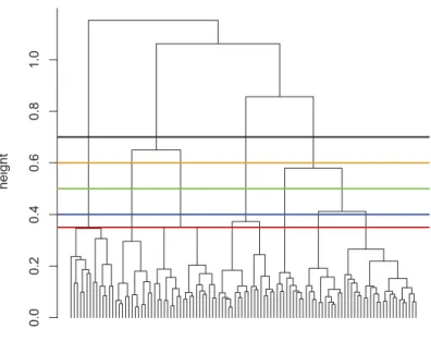
Hierarchical clustering (Figure 4) was performed on the samples based on the dissimilarities of their species compositions. Cluster membership of the samples is expected to be dependent on their stratigraphic position. Increasing the number of groups produces consistent stratigraphic units up to seven groups, which is suggested as the optimal grouping by the KGS penalty function. Four groups were observed at the cutting height of 0.7, five groups at 0.6, six
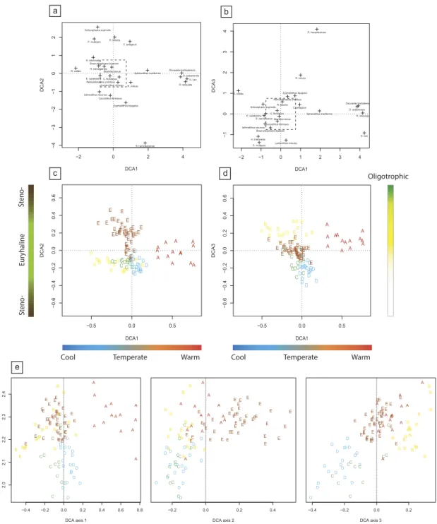
groups at 0.5, seven groups at 0.4 and nine groups at 0.35. However, the difficulty of interpretation rises with the number of phases and the number of outlined units is somewhat arbitrary, as the compo- sitional transition in these communities may unfold in a rather gradual manner. Therefore, we decided to rely on a coarser cluster- ing with five groups, which we hereafter refer to as assemblages, identified in the dendrogram at a cutting height of 0.6. These groups are designated from bottom to top as Assemblage A through E, translated into Phases A through E in a temporal sense. The only exceptions are the samples from 423.6 to 405 m, indicated as parts of thefifth cluster, Assemblage E. Linear discri- minant analysis confirmed the grouping, and assigned these out- lying samples to Assemblages B and D, respectively, where their respective neighbouring samples are placed. The difference between the assemblages is also evident from the results of DCA. The variance explained by thefirst three axes are 43%, 26% and 17%, respectively, showing the relationship between both the strati- graphic units and the species (Figure 5(a,b)). Although the species are more widely spread along the axes than the samples, the pre- viously outlined assemblages form clearly distinguishable sets in both plots (Figure 5(c,d)). Comparison with Shannon’s index of diversity shows that only DCA2 and DCA3 area influenced by sample diversity (Figure 5(e)), Spearman’s rank-order correlation coefficients are 0.6 and 0.57, respectively, both with p < 10−4), whereas DCA1 is not (p= 0.99).
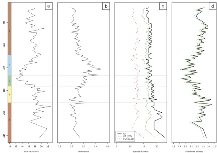
Although changes in abundance and diversity may be easier to identify than compositional changes, they are also best eval- uated using the framework of the five assemblages that mark successive phases established by multivariate analyses (Figure 6).
Abundance decreases markedly in Phase C and drops to its minimum, then continuously increases back to a stable level
Figure 2.Stratigraphic log of the studied interval of the Cserépváralja-1 drillcore (modified after Ozsvárt et al.2016), showing the distribution of the identified calcareous nannoplankton species. Black arrows indicate the studied samples.
through Phase D confirmed by Shannon’s entropy. Although total abundance is maintained in Phase E, it remains signifi- cantly lower than the starting levels in PhaseA(Wilcoxon rank- sum test:p= 2.2 × 10⁻⁴). The increase in total abundance curve after its low point in Phase C is coupled with increased dom- inance. The number of species in a sample remains relatively constant in the section but there is a noticeable shift to lower diversity in Phase D. Sampling standardisation only slightly modifies the raw diversity curve, and the shift is most apparent using the SQS method.
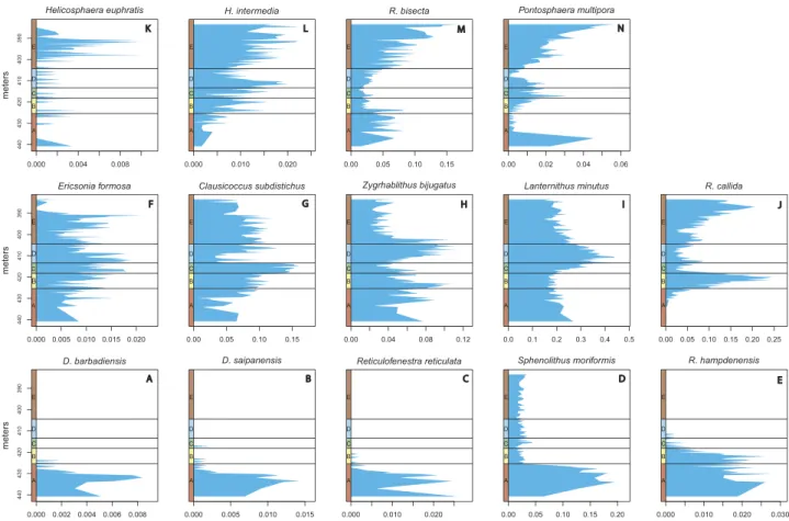
Nannoplankton occurrence and abundance-distribution data were also analysed by constructing abundance curves of individual species (Figure 7). Only the most characteristic 14 species were selected from a total of 29. Three main groups are distinguished
and characterised by taking into consideration the known ecologi- cal preferences of studied species (see next section) and the results of DCA. Thefirstfive curves (bottom row inFigure 7) illustrate species with peak abundance in Phase A. The next five curves (middle row) show more heterogeneity but pertain to species with peak abundance in either Phase B, C orD. The remaining four curves (top row) display species abundance-distribution patterns with maxima during PhaseE.
Palaeoecology
The distribution and association of nannoplankton species primar- ily depend on temperature, salinity, the availability of nutrients and light. We build our assessment of the ecological requirements of the
a b c d
e f g h
i j k l
m n o p
Figure 3.Cross-polarised light photomicrographs of selected biostratigraphically and/or palaeoecologically significant calcareous nannofossil taxa. (a)Discoaster barbadiensisTan.
(b)Discoaster saipanensisBramlette & Riedel. (c)Reticulofenestra reticulata(Gartner & Smith) Roth & Thierstein. (d)Sphenolithus moriformis(Brönnimann & Stradner) Bramlette &
Wilcoxon. (e)Reticulofenestra hampdenensisEdwards. (f)Ericsonia formosa(Kamptner) Romein. (g)Clausicoccus subdistichusPrins. (h–i)Zygrhablithus bijugatus(Deflandre in Deflandre & Fert) Deflandre. (j-k)Lanternithus minutusStradner, (l)Reticulofenestra callidaPerch-Nielsen. (m)Helicosphaera euphratisHaq (N)Helicosphaera intermediaMartini. (o) Reticulofenestra bisecta(Hay, Mohler & Wade) Bukry & Percival. (p)Pontosphaera multipora(Kamptner ex Deflandre in Deflandre & Fert Roth. The scale bar is 10 µm.
encountered taxa (Table 1) on the studies of Báldi-Beke (1984) and Nagymarosy (1992), who outlined groups in the Eocene and Oligocene assemblages from Hungary on the basis of similar eco- logical requirements. We also relied on the fundamental works on coccolithophores by Bukry (1974), Perch-Nielsen (1985), Winter and Siesser (1994), Bown (1998) and Thierstein and Young (2004), as well as more recently published comparative studies from Antarctica (Villa et al. 2008), Tanzania (Dunkley Jones et al.
2008), Greece (Maravelis and Zelilidis 2012), Italy (Violanti et al.
2013), Romania (Melinte2005), and Slovakia (Soták2010). In other
studies (Schneider et al.2013; Bown and Young2019) multivariate analyses suggest that assemblages are significantly perturbated in the shelf region compared to the open sea. Therefore, the fourth category focuses on this parameter in the ecological summary.
Based on literature data, 13 out of 23 species can be confidently assigned to a temperature preference class (Table 1,Figure 8(a)).
The proportion of taxa with colder water preference started to increase in PhaseB, reaching nearly 80% in PhaseC, after which their abundance decreases gradually in Phase E, contrary to the trajectory of taxa with tolerance for brackish water (Figure 8(b)).
0.00.20.40.60.81.0
Ward's method, Bray−Curtis distances
samples
height
0 2 4 6 8 10
440430420410400390380
stratigraphic consistency
clusters numbered from the bottom
meters in the borehole
0.35 cutting height 0.4 cutting height 0.5 cutting height 0.6 cutting height 0.7 cutting height A
B C D E
0 2 4 6 8 10
440430420410400390380
Figure 4.Results of the cluster analysis using Bray–Curtis differences and Ward’s method. (a) Dendrogram of the clustering showing cuts at different heights. (b) Stratigraphic consistency of the grouping achieved at different cutting heights. The x-axis indicates the integer ID value of the sample group and the maximum of each curve indicates the total number of groups in that particular grouping. Decreasing the cutting height from 0.55 progressively increases the number of groups disintegrating AssemblageEin a gradual way.
The proportion of the six brackish and euryhaline salinity indicator species remains relatively constant throughout most of the section, but in AssemblageEthe stress-tolerant forms become a significant component. Taxa preferring shelf habitat show an increasing trend until PhaseD, which reverses in the middle of this phase (Figure 8 (c)). This change is close to the lithostratigraphic boundary between Buda Marl and Tard Clay formations.
The groups revealed by multivariate data analyses are charac- terised in terms of ecological indicator taxa as follows: Assemblage A includes open marine, oligotrophic, oceanic forms, preferring mainly tropical-subtropical climate and normal salinity level. Its most characteristic taxa areDiscoaster barbadiensis, D. saipanensis
and D. tanii; others with similar ecological requirements are Sphenolithus moriformisandReticulofenestra reticulata.
Assemblage B includes open marine, oligotrophic, oceanic forms, preferring temperate surface water temperature and normal salinity level. Significant taxa are Reticulofenestra callida and R. hampdenensis. The differing abundance patterns of these forms suggest the possibility of subdivision within this phase characterised by cold-adapted taxa.
Characteristic taxa in AssemblagesCandDpreferred cool surface water but the same as in AssemblageB, with regard to preference for trophic level and salinity. However, the highest proportion of cold- adapted taxa is observed in AssemblageC. High values in ecological
a b
c
e
d
−0.4 −0.2 0.0 0.2 0.4 0.6 0.8
2.02.12.22.32.4
DCA axis 1
Shannon's entropy
A A
A A A
A
A A A A
A
A A A
B
B B
B B
B B
B B B
B B BB B
B
B B B
CC C
C
C C C
C
C CC
C
D D
D D
D D
D D D
D
D D
DD
D D
D D D E
D E
E
E E E
E E E
EE E E E
E E E E E E E
E E
EE E
E E E
E E
E E E
E E
E E E
E
E E
E
DCA axis 2 A
A
A
A A
A
A A A A
A
A A A
B
B B
B B
B B
B B
B
B B B B
B B
B B B
CC C C
C C C
C
C CC
C
D D
D D
D D
D D D D
D D
D D
D D
D D D
E
D E E
E E E
E E
E
E E
E
E E
E E E E
E
E E
E E EE
E
EE E E E
EE E
E E E E E E
E E
E
−0.2 0.0 0.2 0.4
DCA axis 3 A
A
A A A
A
A A A A
A
A A
A
B
B B
B B
B B
BB B
B B
BBB B
B B B
CC C
C
C C C
C
C CC
C
D D
D D
D D
D D
D D
D D
DD
D D
D D
D E
D E
E
E E
E
E E E
E E
E E E
E E E
E E EE
E E
E E
E
E E
E E E EE
E E
E E
E E E
E E E
−0.4 −0.2 0.0 0.2
Figure 5.(a) Detrended Correspondence Analysis (DCA) ordination of nannofossil species and samples, where letters indicate the assignment of a sample to one of the assemblagesAtoE. (a) Distribution of species along axes DCA1 and DCA2. (b) Distribution of species along axes DCA1 and DCA3. (c) Assemblages along axes DCA1 and DCA2. (d) Assemblages along axes DCA1 and DCA3. (e) The relationship between DCA axes and Shannon’s index of diversity (raw). Only DCA2 and DCA3 are associated with sample diversity.
dominance metrics distinguish these assemblages from both older and younger ones. Characteristic taxa include Reticulofenestra umbilicus, R. minuta, R. oamaruensis, Clausicoccus subdistichus, Zygorhablithus bijugatus, Lanternithus minutus, Blackites tenuis, Ericsonia formosa, Coccolithus pelagicus, C.floridanusandIsthmolithus recurvus.
AssemblageEincludes more oceanic forms than shallow marine or upwelling zone dwellers. The dominant species preferred cool climate and were able to tolerate decreased salinity and increased terrestrial influx.
Species evenness of AssemblageEreturns to the level of AssemblageA.
Marker taxa includeHelicosphaera euphratis, H. intermedia, R. bisecta, Pontosphaera multiporaandBraarudosphaera bigelowii.
Discussion Biostratigraphy
In the previous study of Báldi et al. (1984), a > 25 m thick interval was considered for the position of the Eocene/Oligocene boundary in the core, from 429 m to 402.2 m. According to our results, the zone boundary CNE20/21 is drawn at 427.7 m, based on the last common appearance ofDiscoaster barbadiensisandD. saipanensis.
The acme of Lanthernithus minutus and Zygrhablithus bijugatus begins at 421 m and 426.5 m, respectively, and these events are commonly registered in Zone CNE21, providing regional con- straints for drawing the zone boundary in the core. The well- defined zone boundary between CNO1 and 2 is found at 391 m,
based on the last appearance ofEricsonia formosa. Zone NP21 is known to straddle the Eocene-Oligocene boundary by Martini (1971). The revised biozonation (Agnini et al.2014) could precisely define the position of the series boundary by the Base common of Clausicoccus subdistichus, at 418 m in this study.
The composition of calcareous nannoplankton assemblages is controlled by environmental parameters such as seawater tempera- ture and salinity; therefore, different zonal schemes have been developed for high- and low-latitude marine successions.
Moreover, periodically or permanently isolated marine basins (e.g. the Paratethys) are characterised by different events related to migration or endemic evolution. Thefirst and last appearance data are complementary to those used in the standard zonation. The EOB is placed in the lower part of Zone NP21, based on geogra- phically widely separated studies from Antarctica (Villa et al.2008), Tanzania (Dunkley Jones et al.2008) and the Western Carpathians (Soták2010). However, different placements of the EOB from other regions prove that aligning nannoplankton biostratigraphy with chronostratigraphy is controversial. In the Thrace Basin, a forearc basin of the eastern Balkan region, the EOB is drawn at the top of NP20 zone (LOD ofDiscoaster saipanensis) (Maravelis and Zelilidis 2012). In contrast, the EOB is defined in the upper part of NP21 zone in the Eastern Carpathians (Melinte2005). Although there are different opinions on the correlation of the standard nannoplank- ton zonation, we follow here the prevailing view of placing the EOB within the lower part of Zone NP21 (Bown1998; Dunkley Jones
average number of specimens in a field of view
meters
10 12 14 16 18 20 22
440430420410400390
A B C D E
10 12 14 16 18 20 22
440430420410400390
dominance
0.1 0.2 0.3 0.4 0.5
species richness full
CR (200) SQS (0.95)
5 10 15 20
Shannon's entropy 1.8 1.9 2.0 2.1 2.2 2.3 2.4 2.5 total abundance
a b c d
Figure 6.Stratigraphic changes of abundance and diversity of nannoplankton assemblages through PhasesAtoE. (a) Total abundance of the studied coccolithophores.
Average number of specimens in the studied samples. (b) Dominance values in the studied samples. Note that the number of specimens decreases markedly in PhaseC, followed by an increase of dominance in PhaseD. (c) Species richness in the studied samples. Thick solid line indicates the observed species richness, thin green line indicates standardised richness using classical rarefaction (CR) and dotted lines indicate standardised richness using the SQS method. Note that the richness aspect of diversity remains relatively constant through the section. (d) Shannon’s index of diversity in every sample. Thick solid line denotes raw patterns; thin green line represents values calculated with classical rarefaction.
Helicosphaera euphratis
A B C D E
0.000 0.004 0.008
440430420410400390
meters
H. intermedia
A B C D E
0.000 0.010 0.020
R. bisecta
A B C D E
0.00 0.05 0.10 0.15
Pontosphaera multipora
A B C D E
0.00 0.02 0.04 0.06
Ericsonia formosa
A B C D E
0.0000.005 0.010 0.015 0.020
440430420410400390
meters
Clausicoccus subdistichus
A B C D E
0.00 0.05 0.10 0.15
Zygrhablithus bijugatus
A B C D E
0.00 0.04 0.08 0.12
Lanternithus minutus
A B C D E
0.0 0.1 0.2 0.3 0.4 0.5
R. callida
A B C D E
0.00 0.05 0.10 0.15 0.20 0.25
D. barbadiensis
A B C D E
0.000 0.002 0.004 0.006 0.008
440430420410400390
meters
D. saipanensis
A B C D E
0.000 0.005 0.010 0.015
Reticulofenestra reticulata
A B C D E
0.000 0.010 0.020
Sphenolithus moriformis
A B C D E
0.00 0.05 0.10 0.15 0.20
R. hampdenensis
A B C D E
0.000 0.010 0.020 0.030
A B C D E
F G H I J
K L M N
Figure 7.Abundance distribution of paleoecologically significant taxa. (a)Discoaster barbadiensisTan. (b)Discoaster saipanensisBramlette & Riedel. (c)Reticulofenestra reticulata(Gartner & Smith) Roth & Thierstein. (d)Sphenolithus moriformis(Brönnimann & Stradner) Bramlette & Wilcoxon. (e)Reticulofenestra hampdenensisEdwards. (f) Ericsonia formosa(Kamptner) Romein. (g)Clausicoccus subdistichusPrins. (h)Zygrhablithus bijugatus(Deflandre in Deflandre & Fert) Deflandre. (i)Lanternithus minutus Stradner, (j)Reticulofenestra callidaPerch-Nielsen. (k)Helicosphaera euphratisHaq (l)Helicosphaera intermediaMartini. (m)Reticulofenestra bisecta(Hay, Mohler & Wade) Bukry & Percival. (n)Pontosphaera multipora(Kamptner ex Deflandre in Deflandre & Fert) Roth.
0.4 0.5 0.6 0.7 0.8 0.9 1.0
440430420410400390
proportion of cold water forms
meters
real data simulation A
B C D E
0.4 0.5 0.6 0.7 0.8 0.9 1.0
440430420410400390
0.00 0.01 0.02 0.03 0.04
440430420410400390
proportion (specimens) of brackish forms
meters
A B C D E
0.00 0.01 0.02 0.03 0.04
440430420410400390
0.1 0.2 0.3 0.4 0.5
440430420410400390
proportion of forms with shelf−preference
meters
species specimens
A B C D E
0.1 0.2 0.3 0.4 0.5
440430420410400390
a b c
Figure 8.Environmental changes in the section revealed by the distribution of taxa with inferred palaeoecological preferences. (a) Proportion of specimens of species with a preference for cold waters. Note that Phase C and D are characterised by more abundant cold water forms. The grey lines indicate simulation results from 1000 trials, solid line marks the mean, whereas dashed lines mark 1.96 × the standard deviation of the trials. As the randomisation increases the total proportion of cold water forms, the average line of the simulations is shifted away from the real data. Although the confidence intervals are broad, the upper ones in some samples from unit A are lower than the lower confidence intervals of some samples in unit C and D, indicating a significant shift in the proportion of cold water taxa. (b) Proportion of specimens of species with a preference for brackish waters. (c) Proportion of species (blue line) and specimens (black line) with a preference for shelfal habitats.
et al.2008; Villa et al.2008), the boundary of CNE21 and CNO1 (Agnini et al. 2014), corresponding to the transition from Phase Bto PhaseCin the CSV-1 core.
Previously, the EOB in the CSV-1 core was also determined by foraminifer biostratigraphy, indicated by the last appearance (LAD) of Subbotina linapertaand thefirst appearance (FAD) ofPseudohastigerina naguewichiensisandChiloguembelina gracillima(Báldi et al.1984). Using a chemostratigraphic approach, Ozsvárt et al. (2016) correlated the δ18O curve of CSV-1 with the global stable isotope records, identifying positive peaks probably equivalent of EOT-1 at 410 m, EOT-2 at 407 m and Oi-1 at 405 m. Nevertheless, we suggest a lower position for EOT-1 subevent in this section. Step 1 as thefirst step within the overall δ18O shift during this interval should be placed in the upper Eocene, close to the EOB (Dunkley Jones et al.2008). Also, the Oi-1a subevent could be positioned at 395 m based on the previous measured regional (Ozsvárt et al.2016) and global (IODP database)δ18O stable isotope results.
The moderate preservation in the lower part of Buda Marl Formation may suggest that the lowest total abundance of nanno- plankton in PhaseC linked to the lack of coccoliths rather than environmental control. But the preservation of coccoliths in the upper part of Buda Marl is good, even excellent therefore the environmental change has to be the primary force.
Palaeoecology
Thefive phases distinguished by cluster analysis are best interpreted as the response of nannoplankton assemblages to local environmen- tal changes. The validity of the grouping is well supported by the DCA and the differences are further illustrated by the abundance and diversity curves. The main challenge is to identify which environ- mental parameters are the primary drivers of the observed trends.
In the DCA results (Figure 5), thefirst axis (DCA1) is inferred to reflect the temperature changes during the studied time inter- val. The DCA2 is associated with changes in salinity level. But the DCA3 axis is more difficult to identify as single parameters controlling the nannoplankton distribution. It may represent combinations of several factors such as nutrient level and range of the light source in the photic zone. The groups which preferred cool, temperate or warm surface water are well separated using DCA ordination on the basis of both the distribution of species (Figure 5(a,b)) and assemblages (Figure 5(c,d)). Based on two forms (Helicosphaera euphratis and H. intermedia) that are thought to have tolerated a brackish water environment and two forms (Reticulofenestra bisectaandPontosphaera multipora) which show similar behaviour we can identify a stenohaline and a euryhaline association. There is a hardly recognisable pattern
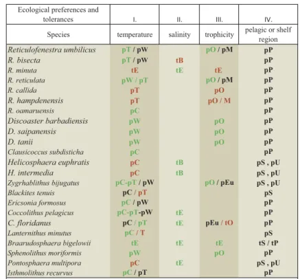
Table 1.The ecological preference and tolerance of the chosen 23 taxa based on published results. We relied on the fundamental works on coccolithophores by Bukry (1974), Perch-Nielsen (1985), Winter and Siesser (1994), Bown (1998) and Thierstein and Young (2004), as well as more recently published comparative studies from Antarctica (Villa et al.2008), Tanzania (Dunkley Jones et al.2008), Greece (Maravelis and Zelilidis2012), Italy (Violanti et al.2013), Romania (Melinte2005), Slovakia (Soták2010) and Hungary (Báldi-Beke1984; Nagymarosy1992). The fourth category focuses on the shelf region compared to the open sea (Schneider et al.2013; Bown and Young2019). Black-coloured letters indicate information based on published ecological data, green colour shows the confirmed published data in this study, brown colour suggests additional preferences and tolerances for taxa with no published predilection.
Ecological preferences and
tolerances I. II. III. IV.
Species temperature salinity trophicity pelagic or shelf region
Reticulofenestra umbilicus pT / pW pO / pM pP
R. bisecta pT / pW tB pP
R. minuta tE tE tE pP
R. reticulata pW / pT pO / pM pP
R. callida pT pO pP
R. hampdenensis pT pO / M pP
R. oamaruensis pC pP
Discoaster barbadiensis pW pO pP
D. saipanensis pW pO pP
D. tanii pW pO pP
Clausicoccus subdisticha pC pP
Helicosphaera euphratis pC tB pS , pU
H. intermedia pC tB pS , pU
Zygrhablithus bijugatus pC-pT / pW pO / pEu pS , pU
Blackites tenuis pC / pT pS
Ericsonia formosus pC / pW pP
Coccolithus pelagicus pC-pT-pW tE pP
C. floridanus pC / pT tE pEu / tO pP
Lanternithus minutus pC / T pS
Braarudosphaera bigelowii tE tE tE tS / tP
Sphenolithus moriformis pW pO pP
Pontosphaera multipora pC tE pS , pU
Isthmolithus recurvus pC / pT pP
p=preference, t=tolerance, C=cool surface water like, W=warm, T=temperate, E=eurytherm,euryhaline,eurytrophic, B=brackish, O=oligotrophic, M=mesotrophic,
Eu=eutrophic, U=upwelling zone, P=pelagic, S=shelf region blackpublished ecological data.
greenconfirmed in this study.
brownnew suggestions based on this study.
based on the distribution of species related to DCA1-DCA3 (Figure 5(a,b)), despite the distribution of assemblages (Figure 5 (c,d,e)). Assemblage A andB preferred oligotrophic conditions.
AssemblageCandDmay have responded to a regional volcanic activity associated with tuffdispersion in the surface water result- ing in limited light source for the algae.
To facilitate more detailed ecological interpretation, we studied the abundance and diversity at both the assemblage and species level (Figures 6–8). Changes in total abundance (Figure 6(a)) and the dom- inance within the assemblages (Figure 6(b)) help reconstruct the local evolution of the nannoflora. The combined effect of global cooling event and local environmental changes is already reflected in Phase B by a decrease in the number of specimens, which reached a minimum in PhaseC. In PhaseE, the composition of theflora became more balanced again, following the rebound of abundance in PhaseD.
There are no dominant forms in PhaseAandBbut dominance values start increasing and reach a peak in PhaseCandDwhen only very few taxa (notably Zygrhablithus bijugatus and Lanternithus minutus) tolerate the environmental change. An event when holo- coccoliths rise to dominance must have represented unusual con- ditions such as the development of an upwelling current.
The raw richness displays virtually no change after some volatility in PhaseA(Figure 6(c)). However, normalised diversity shows a slightly negative shift in PhaseD, which is also observed in other studies from the early Oligocene (Dunkley Jones et al.2008).
As a single coccolithophore individual might be composed of multi- ple elements, it is questionable whether the ranked-abundance distribu- tions of the sampled specimens provide an accurate representation of the individual-level species distributions (Figure 7). The ecological meaningfulness of the relatively small changes in the observed species distributions is questionable; therefore, we refrained from their inter- pretation at face value. However, regardless of how the multiple repre- sentations of an individual modify the species abundance distributions, the relative proportion of forms with different environmental affinities should not be affected significantly and should yield a meaningful signal through time. The abundance curves of different nannoplankton species highlight their ecological preference or tolerance based on previously published opinions (Table 1) and the results of the DCA (Figure 5).
Species are grouped and arranged in rows inFigure 7according to their main ecological constraints. Thefive curves in the bottom row inFigure 7(a–e) illustrate species that preferred warm surface waters and oligo- trophic conditions. The marker species of Discoaster and Reticulofenestra reticulataoccupied similar habitats.Sphenolithus mor- iformisalso preferred elevated SST, but during the cooling event, other ecological traits might have helped its survival. One species in each of the three groups, shown in the last panel in each row (Figure 7(e,j,n)), differs from the others in its abundance distribution pattern and, by inference, in some key aspect of its ecology. The disappearance ofReticulofenestra hampdenensisis not recorded in PhaseAonly later, in PhaseC. This species was probably less sensitive to SST changes and its decline may have been related to subsequent changes in the nutrient level instead or linked to a limited light source resulting from tuff dispersion of Palaeogene magmatism. Five curves shown in the middle row (Figure 7(f–j)) pertain to species whose main shared feature was a cold climate preference. The last common occurrence of marker speciesEricsonia formosais well defined at 391 m. The acme ofClausicoccus subdistichus is recorded in PhasesB–Ebut the Base common of this taxa could be at 418 m, close to the EOB. Zygrhablithus bijugatus and Lanternithus minutusare dominant in PhaseCandD(Figure 7(h, i)). The dominant presence of holococcoliths requires unusual conditions. Both studied taxa preferred colder surface temperatures and cooling climate is not likely to affect their abundance as much as the other species. The shelf region was also preferred by these taxa, indicating that this interval was probably related to an upwelling current. Because of their unique crystal
structure (Cros et al.2000), holococcoliths may also have utilised the limited light source more efficiently, that could have led to their higher abundance.Reticulofenestra callida(Figure 7(j)) shows a unique pattern.
Its abundance remains low during most of the studied interval but in PhasesBandDit shows prominent positive peaks. Thefirst peak may correspond to the transition from warm to temperate oligotrophic conditions that led to a decline of competitors, i.e. species of Discoaster. The second peak is in Phase E when the stress-tolerant species become dominant, suggesting thatR. callidawas also an oppor- tunistic taxon. The remaining four curves (Figure 7(k–n), top row) display the abundance distribution of stress-tolerant forms. Species of Helicosphaera, R. bisecta and Pontosphaera multipora were able to tolerate temperature changes and reduced salinity.Pontosphaera multi- porais also abundant in PhaseA, in agreement with observations that this taxon was also well adapted to warmer waters of near-shore envir- onments (Perch-Nielsen1985; Bown1998). Indeed, palaeobathymetric estimates suggest a shallower depositional environment for the Buda Marl Formation than the overlying Tard Clay Formation, the latter suggested to have formed in a basin of 500–800 m depth (Nagymarosy et al.1995).
The commonly observed overgrowth of calcareous tests, represented by overcalcifying forms, occurs in the lower part of Buda Marl, whereas dissolved forms are more common in the more siliciclastic-rich interbeds.
The quartz grains present in upper Eocene-lower Oligocene strata are probably sourced from the coeval volcanism related to the ongoing Alpine orogeny. The most prominent lithological change, at the boundary between the Buda Marl and Tard Clay Formations, occurs at the transi- tion from PhaseDtoE. The bathyal Tard Clay displays the deepening of Hungarian Palaeogene Basin (HPB) in the early Oligocene (Tari et al.
1993). This change is also manifest in the decreasing trend of species with shelf preference (Figure 8(c)). The increased proportion of taxa tolerating brackish water is not controlled by depth changes but rather by the growing isolation of the water mass (Figure 8(b)).
Thefirst isolation event of the Central Paratethys happened in the early Oligocene (early Kiscellian; Báldi et al.1984). A related salinity decrease was previously suggested on the basis of nanno- plankton assemblages from the top of Zone CNO2, followed by depauperation in Zone CNO3-CNO4, leading to a mono- or duos- pecific nannoflora before and at the onset of bottom water anoxia (Nagymarosy1985). Our results document an earlier onset of major changes, as stress-tolerant species gradually rise to dominance already from the top of Zone CNO1, at the beginning of PhaseE.
The studies of benthic and planktic foraminifera faunas and measurements of carbon and oxygen isotopic compositions of their shells provided additional data from the CSV-1 core (Ozsvárt et al.
2016), enabling their combined evaluation with the nannoflora.
Subdivision to distinct intervals and definition of their boundaries is based on the sudden changes in δ18O, indicative of the early Oligocene cooling, or the increase in the rate of freshwater or terres- trial influx. The temperature signal deduced from δ18O record is confounded by ice-volume or local salinity changes. Ozsvárt et al.
(2016) interpret the oxygen isotopic trends to also reflect a significant freshwater influx precipitated by intensifying monsoon climate.
Therefore, the characteristic species in Assemblage E can tolerate the temperature changes, reduced salinity as well as the increased continental runoffassociated with monsoon activity.
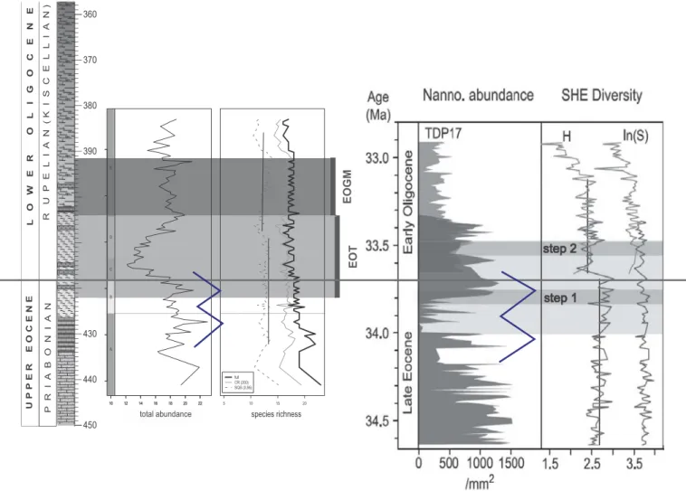
Comparison of the abundance distribution pattern of nannoplankton across the EOT in the CSV-1 core with records from Tanzania (Dunkley Jones et al.2008) reveals remarkable similarities (Figure 9). A W-shaped pattern is observed as the abundance increases in the late Eocene, followed by a decline then another rise before a pronounced negative trend in the early Oligocene. Comparing the diversity curves between isotope steps 1 and 2, a positive shift is present in both our record and that of Dunkley Jones et al. (2008;Figure 9). Our results are similar to this observation with
a slight time lag, probably accounted for by latitudinal differences: low latitude (Tanzania) response to cooling was more immediate than at northern mid-latitude (Central Paratethys). Here the diversity shift found in PhaseDis preceded by the inferred temperature minimum in PhaseCand the decrease in abundance in PhaseB.
Conclusions
This study revealed that the effect of a global cooling event is recogni- sable on the local calcareous nannoplankton assemblages across the EOT in the HPB. Our biostratigraphic subdivision of the CSV-1 drill core documented the presence of Zone CNE21 and Zone CNO1 which include the Eocene/Oligocene boundary. We confirmed that comple- mentary to the standard biozonations (Bown1998; Agnini et al.2014), regional bioevents are helpful in both the biostratigraphic subdivision and successful reconstruction of the environmental history and basin evolution of the Central Paratethys. On the basis of cluster analysis of nannoplankton assemblages, we distinguished five successive phases (AtoE) which are interpreted to reflect the response of the nannoflora to local environmental changes. Abundance distribution of taxa with known environmental preference and DCA analyses yielded palaeoeco- logical insights. In order of decreasing importance, temperature, salinity, and availability of nutrients and light were the environmental para- meters that exerted major control over the abundance and distribution of nannoplankton taxa.
Integrating our nannoplankton-based results with previously published data from foraminifera and stable O and C isotope geo- chemistry (IODP database, Ozsvárt et al.2016), a complex scenario of environmental and biotic changes was reconstructed (Figure 10).
The effects of global climate cooling are overprinted with regional characteristics and superimposed with the influence of isolation of the Central Paratethys basin and regional volcanic activity.
At the beginning of the studied interval, normal salinity condi- tions characterise the shallow bathyal Buda Marl Formation, its nannoplankton assemblages reflect the fully open marine connec- tion of the basin. Prevailing warm and oligotrophic conditions during PhaseAare suggested by nannoplankton and foraminiferan indicator species. The last occurrence of discoasterids is linked to a decline in temperature rather than a change in nutrient availabil- ity. Both the diversity and total abundance show a decreasing trend and overall low values.
PhaseBcontains the start of EOT. Its low-diversity assemblage includes oceanic forms, mostly with the preference of oligotrophic and temperate surface water, allowing to link this interval to the prelude of earliest Oligocene climate cooling. The observed increase in quartz content in these strata may be related to late Eocene volcanism which also probably resulted in tuffdispersion in the photic zone thus limiting the light source for the algae.
During Phase C the cold-adapted species rise to dominance.
Nannoplankton abundance decreases sharply and reaches its
EOTEOGM
U P P E R E O C E N EL O W E R O L I G O C E N E
Figure 9.Comparison of the abundance distribution pattern of nannoplankton across the EOT in the CSV-1 core with records from Tanzania (Dunkley Jones et al.2008) reveals remarkable similarities. A W-shaped pattern is observed as the abundance increases in the late Eocene, followed by a decline then another rise before a pronounced negative trend in the early Oligocene. Comparing the diversity curves between isotope steps 1 and 2, a positive shift is present in both records.