EXAMPLE FOR 2D PLAIN STRAIN DEFORMATION
Author: Dr. István Oldal
6. EXAMPLE FOR 2D PLAIN STRAIN DEFORMATION
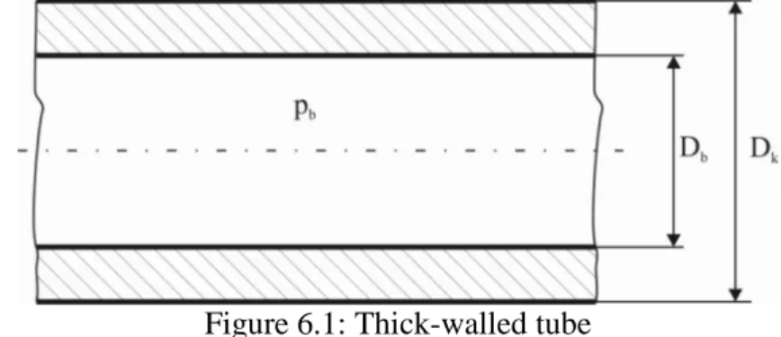
6.1. Thick-walled tube
Let us investigate the solution of a thick-walled tube (shown in Figure 1) with 2D deforma- tion model (Example from Chapter 20.1.4). The tube is pressurized, the outer pressure is neglected.
Figure 6.1: Thick-walled tube Data: Db =60mm, Dk =120mm, pb =30MPa.
6.2. Analytical solution
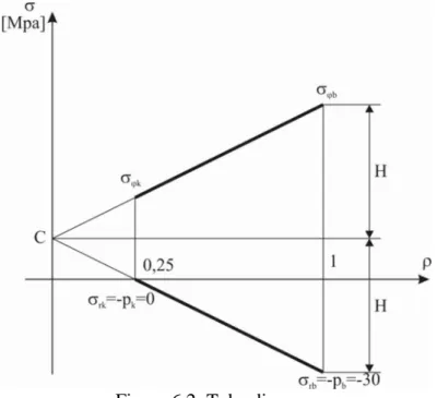
In thick-walled tubes the distribution of the longitudinal stresses is assumed constant, while they change along the radius as a function of quadratic hyperbole. The tube diagrams are commonly plotted as a function of relative reciprocate radius:
2
= rb
ρ r , where:
r: the radius of the tube (variable), rb: the internal radius of the tube.
In our case the number of ρk – considering the external and internal radius – is:
25 , 30 0 60 2
2
=
=
=
b k
k r
ρ r ,
1
2
=
=
b b
b r
ρ r .
According to these numbers the tube diagram is shown in Figure 6.2):
The radial stress in the external and internal wall equals the external and internal pressure.
At ρb =1 we calculate σrb =−30MPa stress while at ρk =0,25 the stress is σrb =0MPa. By connecting these points we obtain the radial stress distribution. Atρ=0 this linear function intersects and determines the value of C . The following proportionality can be derived from the linear function and the two triangles::
rb k b k
C ρσ ρ
ρ = − .
From this we can conclude that:
MPa MPa
C
k b
k
rb 10
25 , 0 1
25 ,
30 0 =
⋅ −
− =
=σ ρ ρ ρ and
MPa C
H = +σrb =40 .
The radial and longitudinal stresses as a function of ρ: ρ
ρ
σr =C−H =10−40 and ρ ρ
σϕ =C+H =10+40 .
The unknown tangential stresses:
MPa H
C b
b = + ρ =10+40⋅1=50
σϕ ,
MPa H
C k
k = + ρ =10+40⋅0,25=20
σϕ .
The axial stresses, depending on whether the tube is open or closed, take the value of 0 or constant C.
6.3. Solution by ANSYS Workbench 12.1 program
In order to solve this specific problem – after starting the program – we have to choose the type of the problem in the project menu. In our case, we wish to carry out a strength check in static condition. Thus we choose the Static structural line (see in Figure 6.3). The selec-
Figure 6.2: Tube diagram
tion can be carried out either by double-clicking or dragging the chosen mode into the white field by holding on the left-click button. After the selection, the requested analysis mode appears in the Project Schematic (see in Figure 6.3.b).
As the window appears, we can specify a name for the task. The window includes six op- tions. By opening the Engineering Data the material constants can be set or modified. This program does not demand to set the material constants, but we have to aware that in this case, it operates with the default settings which are linear, elastic structural steel. By dou- ble-clicking on Geometry, the program starts the geometry module where we are able to draw, modify or import the investigated structure. By double-clicking on Model, we open the finite element module which involves and activates the Setup, Solution and Result op- tions. In the Project Schematic we can always see the conditions of the separated modules, since the ready modules are presented by green pipes, the missing ones with yellow ques- tion mark, while the false ones with red exclamation mark. The ready but not-yet-executed modules are marked with yellow lightning icons.
6.3.1. Geometry modeling
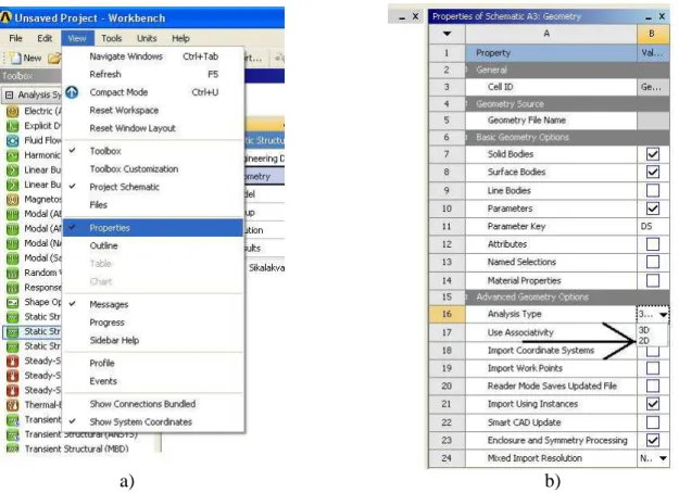
A planar deformation problem begins with the 2D modeling. This can be set before or after drawing the geometry in the Project Schematic. By clicking on Geometry, we can see the Property window on the left side of the screen and in its 16th line we can define the default
a) b) Figure 6.3: Project Schematic window
3D option to 2D (see in Figure 6.4.b). If the Properties of Schematic window is not visible, then if we click on View/Properties menu (see in Figure 6.4.a) it becomes visible.
After setting the dimension of the problem, we start the Design Modeler menu by double- clicking on Geometry in the Static Structural window. First of all, we have to define the unit (see in Figure 6.5).
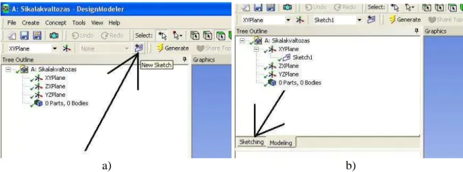
The Design Modeler – similar to other 3D modeler software – builds up the models from layers and sketches by modifying them. Before drawing a sketch, we have to choose a plane to work with. The default plane, if we do not choose anything else, is the xy plane.
2D problems are compulsory drawn in this plane, since the program cannot define other planes in case of two-dimensional modeling. To draw a sketch, we have to click on New sketch icon (see in Figure 6.6.a), then in the left window – as a branch of the defined plane – Sketch1 appears. Let us now click on Sketching tab (see in Figure 6.6.b).
a) b) Figure 6.4: Setting the dimension of the problem
Figure 6.5: Selecting unit
In order to have a better view over the sketch, we change our point of view from the de- fault axonometric view to a view which is perpendicular to the sketch by clicking on the icon shown in Figure 6.7.
Let us select Circle command in Draw window (Figure 6.8.a) and draw two concentrical circles, then with Dimensions/Radius command (Figure 6.8.b) we appoint the two circles and we set the radius to 30mm and 60mm in Details View window.
a) b) Figure 6.6: Making new sketch
Figure 6.7: Setting the View perpendicular to the sketch
a) b) Figure 6.8: Sketch menu
If we wish to solve the problem as a quarter circle – by utilizing the symmetry – instead of a full circle, then with command Draw/Line (Figure 6.8.a) we draw two lines at the quarter circles and we cut off the outlining parts with Modify/Trim command (Figure 6.9.a).
Now we have to make surfaces on the complete sketch (Figure 6.9.b). By clicking on Mod- eling tap (Figure 6.10.a) we exit the sketch drawing and then we execute Concept/Surfaces from sketches command by clicking on it (Figure 6.10.b).
After executing the command, the Details of SurfaceSk1 window appears on the left side of the screen (Figure 6.11).
a) b) Figure 6.9: Sketch menu and the complete sketch
a) b) Figure 6.10: Exiting Sketch and making surfaces
We can see the name of the surface – which we are about to make – in the window (the program automatically creates a name). In the second line, we can choose the sketch that we use for making the surface. The selection can be carried out by either clicking on the chosen line of the sketch or clicking on the appropriate branch of the tree structure. In our case there is only one sketch, thus it is automatically selected, but in all the other three cases we have to accept our decision by clicking on Apply in Base Objects menu (Figure 6.11.a). The other options stay as default, we execute the Generate command (Figure 6.11.b) and our surface is already generated and appeared in the last branch of the tree structure as Surface Body (Figure 6.12). Then, we return to the project menu.
6.3.2. Finite Element Simulation
In the project module, by double-clicking on Model (Figure 6.13.) in the Static Structural window, the finite element module (Mechanical) starts. Make sure that you set the module to 2D modeling in the Properties of Schematic window of the Geometry menu (Figure 6.4.b).
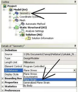
After starting the module, we have to define the type of the 2D problem. By clicking on the Geometry branch of the tree structure, the Details of Geometry window opens, where the options for 3D modeling becomes visible in the 2D Behavior settings (Figure 6.14). Let us select the Plane Strain model. In this case – and in the axis-symmetric case – no other pa- rameters have to be set. In Plane Strain model, we only have to define the thickness of the plate between each surface as parameters.
Figure 6.11: Settings on Surface
Figure 6.12: The generated surface in the tree structure
Figure 6.13: Starting the Finite Element simulation
6.3.3. Meshing
As a first step of modeling, we have to discretize the model by creating a mesh. If we do not set the meshing parameters, the program will create a mesh with the default settings.
This method results rarely optimal mesh.
By right-clicking on the Mesh branch, the parameters of the mesh can be set under the up- coming Insert window. Firstly, we choose the element type with the Method command (Figure 6.15.a).
Figure 6.14: Selection of 2D modeling
a)
b) c) Figure 6.15: Settings of the mesh
In order to execute the command we have to select the body (if it is not the surface of a body but a surface model of a body the Workbench will model it as a body ‘Surface Body’) and then click on Method command (Figure 6.15.a). Then the Details window appears be- low, on the left corner, and we can carry out the settings.
Unlike other finite element programs, not the element type has to be selected, but by defin- ing the parameters of the mesh, the program will automatically select element type fitting to the mesh. In the Method option (Figure 6.15.b) triangular and rectangular elements can be selected. In our case the rectangular elements are the most adequate. The order of the approximate functions (the numbers of the element nodes) can be set in the Element Mid- side Nodes option (Figure 6.15.c). In this specific case the quadratic approximation is needed since the planar model cannot be meshed with linear functions (it is not enclosed by linear lines). Let us select the rectangular element with eight nodes – including the nodes in the middle plane – and click on Kept.
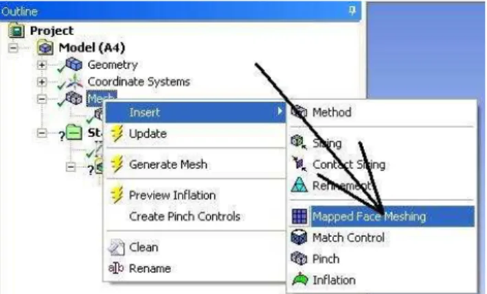
The stress changes along the radius in a thick-walled tube, but not in a constant radius. In order to reduce the numerical errors, we create a mesh by taking into account pattern. By executing the Mapped Face Meshing command (Figure 6.16) we create a structured mesh.
After the command is executed, we have to select the surface and accept it with the De- tails/Apply command. If the geometry is unsuitable for this mesh due to its complexity, then a blue circle appears in the tree structure.
Figure 6.16: Starting the finite element simulation
The program automatically defines the size of the mesh, proportional to the body, but this can modified according to our needs. If we wish to use default mesh size, we can do that in the Details of Mesh/Sizing window. If we want to define different element size at the edges, surfaces, then we have to apply the Insert/Sizing command (Figure 6.17.a). After selecting the command, we have to choose the applicable geometry where we wish to set the size. In our case, this is the inner curve of the quarter circle and the curves of the two radiuses. The selecting has to be switched at the top icon menu (Figure 6.17.b). In the De- tails of Sizing window the selected curves have to be accepted by and the element size – 5 mm – has to be typed into the Element Size option. We must not define size on the outer curve, since the structured mesh will define provide that.
As it was mentioned earlier, we can execute the Generate Mesh (Figure 6.18.a) command and create our mesh (Figure 6.18.b).
a)
b) c) Figure 6.17: Setting the element size
a) b) Figure 6.18: Mesh generation and the complete mesh
6.3.4. Setting the boundary conditions
We can find the boundary conditions by right-clicking on the Static Structural branch and selecting Insert option (Figure 6.19).
In this specific case, two types of boundary conditions must be specified; the internal pres- sure and the symmetry conditions.
The Pressure command can be applied on our model if we wish to specify distributed force system along a line instead of pressure. After defining the model- and model related pa- rameters, the program automatically recalculates the given pressure value.
By the use of the Pressure command, we have to select the inner curve and accept it with Apply command (Figure 6.20). In the Magnitude option we can enter the 30MPa value.
The symmetry is defined by displacement constraints which are applied on the two radius orientated lines. We execute the Displacement command (Figure 6.19) and select the two vertical lines.
Figure 6.19: Boundary conditions
Figure 6.20: Defining the pressure
The selection has to be accepted in the Details of Displacement window by the Apply command, and then the displacement along the x axis is set to zero (Figure 6.21), while the y stays permissible. This method has to be carried out on the horizontal line as well, but there the vertical displacement has to be set to zero.
6.3.5. Results
After setting the boundary conditions the simulation can be executed by the Solve com- mand. The requested results can be displayed after the simulation manually, but if we se- lect which results are we interested about, then these results will automatically displayed after the computation.
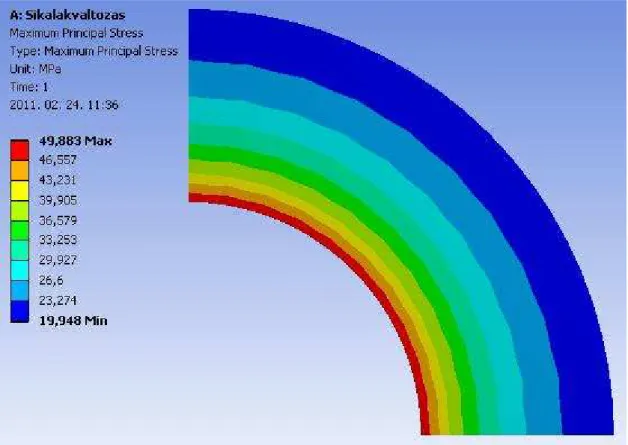
In this specific case, we would like to compute the tangential stresses. In case of pressur- ized tubes or vessels, we know that the principal stresses are radial, tangential or axial ori- entated and the tangential is the highest. Thus we right-click on the Solution branch and we select the Insert/Stress/Maximum Principal option (Figure 6.22).
The computation of the problem can be initiated either by clicking on the Solve icon on the top menu, or right-clicking on the Solution branch and selecting the Solve command (Fig- ure 6.23).
Figure 6.21: Defining the vertical symmetry
Figure 6.22: Displaying the required results
After executing the simulation we can display the required stresses by clicking on Solu- tion/Maximum Principal Stress branch (Figure 6.24).
Figure 6.23: Starting the computation
Figure 6.24: Calculated stresses