Lagrangian Models for Controlling Large-Scale Heterogeneous Traffic
Tam´as G. Moln´ar, Devesh Upadhyay, Michael Hopka, Michiel Van Nieuwstadt, and G´abor Orosz
Abstract— Heterogeneous traffic with a mixture of human- driven and connected automated vehicles is discussed to study how the penetration rate and the control design of connected automated vehicles affect the traffic flow on a large scale.
Continuum traffic models are constructed by incorporating time delays to take into account the reaction time of human drivers and the delays in the control loops of connected automated vehicles. It is shown that Lagrangian delayed continuum models are suitable for studying heterogeneity, introducing delay, and taking into account the on-board traffic data used by the controllers of connected automated vehicles. We show that these models possess realistic stability properties and are capable of capturing the large-scale dynamics of vehicle automation- induced and connectivity-induced heterogeneity.
I. INTRODUCTION
The effect of connected automated vehicles (CAVs) on the safety and mobility of traffic is a central question in today’s transportation research. While vehicles, cities and traffic infrastructure will become increasingly connected in the near term, it is also clear that until full penetration is achieved there will exist a period of mixed traffic. Thus, studying heterogeneous traffic flows is an important research topic.
Traffic flow can be described either by a discrete number of vehicles (discrete models) or by a continuous distribution of vehicles along the highways (continuum models). Continuum models are relevant for studying large-scale networks with a large number of vehicles. They are useful to investigate the effect of the penetration rate of CAVs and the effect of their control design on the large scale. They are also relevant in traffic forecasting and traffic jam prediction.
Traffic flow can be described in Lagrangian framework by tracing the motion of individual vehicles, or in Eulerian framework by observing traffic at fixed locations. The last century put emphasis on Eulerian models [1], [2], as traffic was measured in Eulerian fashion via loop detectors at predetermined locations along the road. Today individual vehicles gather data by GPS (Global Positioning System) and other on-board sensors, providing Lagrangian traffic measurement. Controlling the motion of individual CAVs is also a Lagrangian approach for regulating traffic flow.
Still, most continuum models in the literature are formu- lated in Eulerian framework. They also ignore an essential ingredient: the time delays associated with the reaction time of human drivers and the delays in the control loops of
T. G. Moln´ar and G. Orosz are with the Department of Me- chanical Engineering, University of Michigan, Ann Arbor, MI, USA molnart@umich.edu, orosz@umich.edu
D. Upadhyay, M. Hopka and M. Van Nieuwstadt are with the Ford Research and Innovation Center, Dearborn, MI, USA dupadhya@ford.com, mhopka@ford.com, mvannie1@ford.com
...
n-1 n
n+1 1 0
X(n,t) V(n,t)
0 Lagrangian description
0 x Eulerian description
...
v(x,t) N(x,t) (a)
(b)
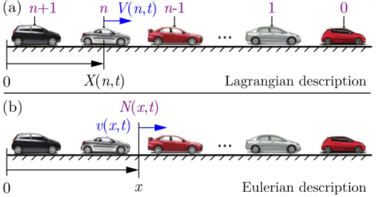
Fig. 1. Illustration of the Lagrangian and Eulerian frameworks for traffic flow description.
CAVs [3]. These delays are related to individual vehicles, not locations. The introduction of delays into continuum models is nontrivial, there are only a few recent attempts in literature [4], [5], [6]. This paper is devoted to a possible approach for constructing delayed Lagrangian continuum models of highway traffic. The stability of the resulting models is analyzed and emphasis is put on modeling the automation-induced heterogeneity of the traffic flow.
II. FRAMEWORKS FOR TRAFFIC MODELING First we discuss the possible choices of independent vari- ables that give the framework for analytical traffic models.
A. Lagrangian Framework
A potential approach to modeling traffic is tracing the motion of individual vehicles, which is referred to as the Lagrangianframework. As illustrated in Fig. 1(a), a vehicle numbernis associated to each vehicle in traffic (withn= 0 being the lead vehicle) and relevant quantities are described as a function of the vehicle numbernand timet. We remark that it is not necessary to restrict this framework to an integer number of vehicles. Quantities at non-integer vehicle numbers represent interpolations between the integer ones, which enables the construction of continuum traffic models.
The most fundamental quantity in this framework is the vehicular positionX(n, t)(measured in m relative to the da- tum att= 0), which can be directly measured by equipping vehicles with GPS. X(n, t) is a monotonically increasing function oftand a strictly monotonically decreasing function of n, since vehicles travel in the direction opposite to their numbering. Note that we assume a single lane scenario where vehicles maintain their order, that is, they do not overtake each other.
B. Eulerian Framework
Another approach for traffic description is the Eulerian framework illustrated in Fig. 1(b). A certain cross section of the road at positionxis selected for observation. Traffic measures are described as a function of the position x and timet. When no vehicle is located at x, the corresponding quantities can be regarded as interpolations between the values related to the two neighboring vehicles.
One essential quantity of this framework is the so-called cumulative flowN(x, t)(measured in vehicles). It indicates the number of vehicles (more accurately, the vehicle number) that reach positionxby timet[7], [8].N(x, t)is a monoton- ically increasing function of t and a strictly monotonically decreasing function ofx, since less vehicles reach positions farther along the road by time t.
C. Transition between the Frameworks
In Lagrangian framework, we use Roman letters to denote traffic measures such as velocityv(n, t)(m/s), traffic density r(n, t)(vehicles/m) and traffic flux Q(n, t) =r(n, t)v(n, t) (vehicles/s). In Eulerian framework, we use Greek letters:
velocity ν(x, t)(m/s), density ρ(x, t) (vehicles/m) and flux ϕ(x, t) =ρ(x, t)ν(x, t)(vehicles/s). From practical point of view, traffic density describes the number of vehicles on a certain highway segment. Here, density is defined locally for each vehicle number or position along the road as explained in Sec. III. Traffic flux indicates the number of vehicles that pass a certain cross section of the highway over a unit time.
The Roman and Greek notations indicate the same physi- cal quantity but as a function of different independent vari- ables. The quantities in one framework can be transformed to the other. Transition from Eulerian to Lagrangian framework is done by considering the cross section xwhere vehiclen is located by the substitutionx=X(n, t). Thus,
r(n, t) =ρ(X(n, t), t),
v(n, t) =ν(X(n, t), t). (1) Similarly transition from Lagrangian to Eulerian framework is achieved by considering the numbernof the vehicle that is located at positionxby the substitutionn=N(x, t):
ρ(x, t) =r(N(x, t), t),
ν(x, t) =v(N(x, t), t). (2) III. CHOICE OF DEPENDENT VARIABLES Below we give the definition of traffic density in the local sense and we discuss other possible measures of traffic flow.
A. Local Definition of Traffic Density
The practical (non-local) definition of traffic density is the number of vehicles distributed on a road segment of unit length. In the Lagrangian description, one may consider the road segment between the positionsX(m, t)andX(n, t)of vehiclesmandn, whence the density becomes the ratio
r(m, t)≈ − m−n
X(m, t)−X(n, t). (3)
Here the negative sign is necessary to force positivity for the density r given the convention that the higher vehicle number is upstream in the traffic flow. For two consecutive vehicles (say n−1 andn), the density is equivalent to the inverse of the distance between them. The local definition of density is obtained by taking the limitm→n. This leads to
r(n, t) =− 1
∂nX(n, t). (4)
In the Eulerian framework, the density definition considers the road segment between the positionsy andx associated with vehicle numbers N(y, t) and N(x, t), respectively.
Density is therefore the ratio
ρ(y, t)≈ −N(y, t)−N(x, t)
y−x (5)
with the negative sign as before to enforce positivity. Taking the limity→xgives the local definition
ρ(x, t) =−∂xN(x, t). (6) B. Choice of a Single or Multiple Dependent Variables
In order to describe the traffic flow, appropriate dependent variables must be selected. In each framework, it is possible to choose a single dependent variable or a combination of multiple variables. In the Lagrangian framework, one may use either the position X(n, t) or the velocity v(n, t) and densityr(n, t), which are related by
∂nX(n, t) =− 1 r(n, t),
∂tX(n, t) =v(n, t).
(7)
Instead of the pair(v, r), one may also use their product, the fluxq, and choose the pair (v, q)or (r, q).
In the Eulerian framework, one may choose the cumulative flow N(x, t) as a single dependent variable or the pair of densityρ(x, t)and flux ϕ(x, t), which are related by
∂xN(x, t) =−ρ(x, t),
∂tN(x, t) =ϕ(x, t). (8) Instead of the pair (ρ, ϕ), equivalent choices could be the pairs(ν, ρ)or(ν, ϕ)with velocityν.
IV. DELAYED CONTINUUM MODELS Hereinafter we derive continuum traffic models from mod- els with a discrete number of vehicles. We put emphasis on including time delays in the models to characterize human reaction time and delays in the control loops of CAVs [3].
A. Benchmark Discrete Model
Discrete models are intrinsically formulated in Lagrangian framework, since they are discrete in variablen. One of the simplest discrete models is the one by Newell and Igarashi et al. [9], [10], [11]. Accordingly, vehiclencontrols its velocity based on the distance from its predecessor vehiclen−1:
∂tX(n, t) =V(X(n−1, t−τ)−X(n, t−τ)). (9)
Function V defines the distance-velocity relationship (also referred to as the range policy in the rest of the paper). It is monotonically increasing: the farther the vehicles move away from each other, the faster they shall travel. The model includes the time delayτ: a given vehicle (with fixed vehicle number n) reacts to the past state of traffic at time t−τ instead of the instantaneous state at timetin order to account for the reaction time of its driver or the delay in its control loop. First we assume identical range policyV and delayτ for each vehicle (eachn), then we address the heterogeneity of traffic (the n-dependency) at the end of this paper.
Model (9) is a first order differential equation in timetthat contains a time delayτ. The model also involves a unit delay in variable n, which arises from the discrete nature of the model. If the unit delay is approximated, one may obtain a continuum counterpart of the discrete model. Below we give two different approaches for constructing continuum models from the discrete model (9). These approaches can be applied for other (possibly higher order) discrete models as well.
B. Delayed Lighthill-Whitham-Richards (LWR) Model First, let us consider the approximation
X(n−1, t)−X(n, t)≈ −∂nX(n, t). (10) Substitution into (9) leads to the continuum model
∂tX(n, t) =V(−∂nX(n, t−τ)). (11) Note that keeping higher order terms on the right-hand side of (10) is also possible, but it leads to more complex models; see [12] for a third order case with τ= 0 in Eulerian description. In (11) we consider a first order model supplemented with the identity
−∂tnX(n, t) +∂ntX(n, t) = 0. (12) Later we use this identity to show that (11)-(12) is in fact equivalent to the well-known Lighthill-Whitham-Richards (LWR) model [1], [2], but in the Lagrangian framework with an additional time delay τ. This Lagrangian form can be found in [13] forτ= 0.
First, let us write (11)-(12) in terms of the Lagrangian densityr(n, t)and the Lagrangian velocityv(n, t)using (7):
∂t
1
r(n, t)+∂nv(n, t) = 0,
v(n, t) =V(1/r(n, t−τ)) =V(r(n, t−τ)).
(13) This equation can also be found in [13], [14] for the case τ= 0 and in [5] for τ >0. The first row of (13) can be interpreted as a conservation law for the number of vehicles participating in traffic. The second row defines the speed- density relationship via the monotonically decreasing func- tion V(r) =V(1/r): the denser the traffic gets, the slower the vehicles travel. Equations (9), (11) and (13) show the main difference between discrete and continuum approaches:
discrete models use inter-vehicular distance (difference of positions), while continuum models operate with density (related to thederivativeof positions with respect ton).
Now let us represent the model in Eulerian framework. Let us substitute (1) into (13), carry out differentiations according to the chain rule and finally substitute x=X(n, t). This leads to the classical form of the LWR model in Eulerian framework using the densityρ(x, t)and the fluxϕ(x, t):
∂tρ(x, t) +∂xϕ(x, t) = 0,
ϕ(x, t) =ρ(x, t)V(ρ(x−ξ, t−τ)). (14) The first equation describes the conservation of vehicles on the road. The second equation is the model of traffic dynamics itself: it describes the relationship between flux and density. Due to the delay, the flux depends on a past value of the density at timet−τinstead of the instantaneous value at timet. Timet−τ corresponds to locationx−ξon the highway (not simplyx), whereξ is the displacement of vehiclenover[t−τ, t]. Note thatξis a spatial delay in (14) and it is given below.
Before specifyingξ, we formulate the model in Eulerian framework in terms of the cumulative flow N(x, t)for the sake of completeness. By substituting (8) into (14) we obtain
−∂txN(x, t) +∂xtN(x, t) = 0,
∂tN(x, t) =−∂xN(x, t)V(−∂xN(x−ξ, t−τ)). (15) This formulation can also be found in [7], [13] for the case τ= 0. Notice that similarly to (12) the first row of (15) is an identity. This implies that the definitions (4) and (6) of the densitiesr(n, t)andρ(x, t)ensure the automatic fulfillment of the conservation law of vehicles.
Finally, let us specify the spatial delayξ. The derivation of the Eulerian model (14) from the Lagrangian one (13) results in the following value forξ:
ξ=X(n, t)−X(n, t−τ), (16) which is equivalent to
ξ= Z t
t−τ
v(n,˜t)d˜t . (17) That is, the spatial delayξcan be obtained from the solutions of the Lagrangian models (11) and (13). In Eulerian frame- work, however, eitherN(x, t)or ρ(x, t) andϕ(x, t)should be used to obtainξ. Since timetand positionxcorrespond to the same vehicle number ast−τ andx−ξ, we write
N(x, t) =N(x−ξ, t−τ). (18) Via (8), it can be shown that (18) is equivalent to
Z t
t−τ
ϕ(x,˜t)d˜t= Z x
x−ξ
ρ(˜x, t−τ)d˜x . (19) These equations implicitly define the spatial delay ξ as a function of τ and the statesN(x, t)orρ(x, t)andϕ(x, t).
Note that both Eulerian models, (15) with (18) and (14) with (19), formulate a partial delay differential equation (PDDE) with constant time delay and state-dependent spatial delay. This spatial delay was neglected in the PDDE models of [4], [5]. Since state-dependent delays make the analysis of differential equations significantly more difficult [15], it is more useful to use Lagrangian framework for introducing
delays. This highlights that in fact the classical Eulerian formulation (14) of the LWR model is the least suitable form for including time delays. In Eulerian framework one needs to consider that past events at time t−τ took place at location x−ξ (not simply x) due to the propagation of traffic. In Lagrangian framework, however, delays can simply be added to the model, since vehiclenreacts to the delayed traffic state associated with the same vehicle numbern.
C. A Higher Order Delayed Continuum Model
A more sophisticated continuum approximation of the discrete model (9) can be given as follows. In the literature of delayed dynamical systems, time delays are often approx- imated by first order lags. Using this idea, let us approximate the unitn-delay in (9) with a unit lag. We rewrite (9) as
∂tX(n+ 1, t) =V(X(n, t−τ)−X(n+ 1, t−τ)) (20) and then we use the Taylor series expansion
X(n+ 1, t) =X(n, t) +∂nX(n, t) +1
2∂nnX(n, t) +. . . , (21) which can be truncated after first order. This leads to the following Lagrangian continuum model with unit lag in n:
∂tX(n, t) =V(−∂nX(n, t−τ))−∂tnX(n, t). (22) Note that the difference of positions (the distance) in the discrete model (9) is again replaced by the position derivative (related to the density) in the continuum model (22). In contrast to the delayed LWR model (11), model (22) involves a second order term (∂tnX) as well. This term was produced by the first order lag approximation, which increases the order of the model while removing the delay in n. We will show in Sec. V that this higher order term provides more realistic stability properties for the continuum model.
Similarly to the delayed LWR model (11), it is possible to construct equivalent forms for the continuum model (22).
The Lagrangian form with density and velocity reads
∂t
1
r(n, t)+∂nv(n, t) = 0, v(n, t) =V(r(n, t−τ)) +∂t
1 r(n, t).
(23)
The Eulerian form with density and flux becomes
∂tρ(x, t) +∂xϕ(x, t) = 0,
ϕ(x, t) =ρ(x, t)V(ρ(x−ξ, t−τ)) +∂x
ϕ(x, t)
ρ(x, t), (24) and with the cumulative flow it reads
∂tN(x, t) =−∂xN(x, t)V(−∂xN(x−ξ, t−τ))
−∂x
∂tN(x, t)
∂xN(x, t). (25) whereξis given by (19) and (18), respectively.
Notice that an additional term arises in (22)-(25) compared to the delayed LWR model (11)-(15). In the literature, there are various attempts to specify reasonable additional terms
to the LWR model to get more realistic behavior for its solutions [16], [17], [18], [19]. Here this term was derived from the first order lag approximation of a discrete model.
V. STABILITY ANALYSIS
In this section, we analyze the string stability properties of models (9), (11) and (22). String stability means the attenuation of velocity fluctuations along a chain of vehicles, which is directly related to the mitigation of traffic jams on the highway. That is, string stability is the stability of solutions with respect to n. In order to analyze string stability, we linearize the models and write the equations at the velocity level. Linearization is performed around the uniform flow v(n, t)≡v∗ of constant speed v∗, where the corresponding uniform distanced∗ is given byV(d∗) =v∗ for the discrete model (9), while the uniform density r∗ of the continuum models (11) and (22) satisfiesV(1/r∗) =v∗. Linearization of the discrete model (9) and differentiation with respect to time yields
∂t˜v(n, t) =κ(˜v(n−1, t−τ)−v(n, t˜ −τ)), (26) where v(n, t) =˜ v(n, t)−v∗ denotes the velocity fluctua- tions around the uniform flow and κ=V0(d∗)>0 is the derivative of the range policy. Similarly, the linearized coun- terpart of the continuum models (11) and (22) read
∂t˜v(n, t) =−κ∂n˜v(n, t−τ), (27) and
∂tv(n, t) =˜ −κ∂n˜v(n, t−τ)−∂tn˜v(n, t), (28) respectively, whereκ=V0(1/r∗)>0.
A. String Stability Condition
We analyze string stability by assuming harmonic velocity fluctuations. Note that general velocity fluctuations can also be decomposed into harmonics. Considering fluctuations of angular frequencyω >0, we assume˜v(n, t)in the form
˜
v(n, t) =vampeiωteλ(ω)n, (29) whereλ(ω)determines how the velocity fluctuations prop- agate along a string of vehicles. The real part of λ(ω) determines whether the fluctuations amplify or decay, and it has to be negative for allω >0to guarantee string stability.
The imaginary part of λ(ω) is the wave number, which defines the angular frequency of fluctuations in terms of the vehicle numbern. Note that when physically evaluating the results of continuum models, solutions are considered at integer vehicle numbers only. This implies a sampling with period 1 in terms of the variable n. According to the Nyquist-Shannon sampling theorem, phenomena of period smaller than2cannot be captured by sampling with period1.
Therefore, angular frequencies (wave numbers) above π can be disregarded during string stability analysis, and we formulate the condition for string stability as
<(λ(ω))<0 or |=(λ(ω))|> π, ∀ω >0. (30)
B. String Stability of the Discrete Model
Substitution of the trial solution (29) into (26) gives the characteristic equation of the discrete model (9) in the form
iω=κ
e−λ(ω)−1
e−iωτ, (31) which can be rearranged to
eλ(ω)= κ
iωeiωτ +κ =T(iω). (32) Note thatT(iω) = eλ(ω)is the transfer function between the velocity fluctuations of vehiclen−1andn[20]. Accordingly, the string stability condition (30) can also be written as
|T(iω)|= eλ(ω)
<1, ∀ω >0. (33) Given (32), this condition is equivalent to
2κτsin(ωτ)
ωτ −1<0, ∀ω >0. (34) Forτ= 0, the system is string stable for anyκ. Forτ >0, the critical case ω→0+ gives the largest left-hand side in (34), which implies the following string stability condition for the discrete model (9):
τ <1/(2κ). (35)
C. String Stability of the Delayed LWR Model
Substitution of (29) into (27) gives the characteristic equation of the delayed LWR model (11) in the form
iω=−κλ(ω)e−iωτ. (36) Note that this can also be obtained from the characteristic equation (31) of the discrete model by the approxima- tion e−λ(ω)≈1−λ(ω), which corresponds to (10). Equa- tion (36) can be rearranged to
λ(ω) =−iωeiωτ
κ = 1− 1
T(iω). (37) Equations (30) and (37) imply the string stability condition
sin(ωτ)<0 or ω|cos(ωτ)|
κ > π, ∀ω >0. (38) The case τ= 0, which corresponds to the classical, delay- free LWR model, is marginally string stable, since the left- hand side of the first inequality gives 0. The marginal stability is an essential property of the LWR model due to the hyperbolic nature of the governing PDE. For τ >0, however, (38) is not fulfilled in the critical case ω→0+. Thus the delayed LWR model (11) is always string unstable, regardless the value ofκ.
D. String Stability of the Higher Order Model
Substitution of (29) into (28) yields the characteristic equation of the higher order delayed continuum model (22):
iω=−κλ(ω)e−iωτ −iωλ(ω). (39) The solution for λ(ω)reads
λ(ω) =− iωeiωτ
iωeiωτ +κ=T(iω)−1, (40)
which can also be obtained from (31) by the approximation eλ(ω)≈1 +λ(ω) according to (21). The string stability condition (30) implies
κτsin(ωτ)
ωτ −1<0 or κω|cos(ωτ)|
(κ−ωsin(ωτ))2+ (ωcos(ωτ))2 > π, ∀ω >0. (41)
Forτ = 0, the system is string stable for anyκ, similarly to the discrete model (9). Forτ >0, the critical caseω→0+ is the most restrictive in terms of the first inequality. This leads to the string stability condition
τ <1/κ . (42)
Note that stability condition (42) of the continuum model (22) differs only by a factor of2 from stability con- dition (35) of the corresponding discrete model (9). Recall that (22) was derived by the first order lag approximation of the unit n-delay in (9) using first order expansion in (21).
Higher order terms in (21) could be taken into account similarly. For example, second order expansion gives
∂tX(n, t) =V
−∂nX(n, t−τ)−1
2∂nnX(n, t−τ)
−∂tnX(n, t)−1
2∂tnnX(n, t). (43) In fact, it can be shown that (43) has exactly the same stability condition (35) as the discrete model (9).
VI. CONCLUDING REMARKS
Today’s traffic measurement and control of connected au- tomated vehicles (CAVs) strongly relies on Lagrangian data collected by individuals in traffic, which creates a need for Lagrangian traffic models. We have shown that Lagrangian description is suitable for modeling human driver reaction time and feedback delays in CAVs, while complicated state dependent spatial delays arise in Eulerian models. The La- grangian framework facilitates the construction of delayed continuum models from discrete models, although special care must be taken to obtain realistic stability properties.
Stability analysis revealed that simply adding a delay to the LWR model exhibits string unstable behavior, while introducing higher order terms via approximation of discrete models gives realistic stability conditions. It is even possi- ble to construct delayed continuum models with equivalent stability conditions to those of discrete models.
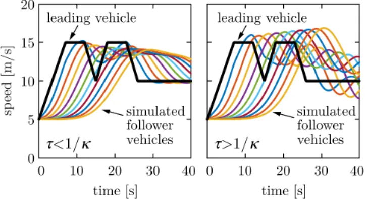
The result of such delayed continuum models is illustrated in Fig. 2, where (22) is simulated. The leader’s speed profile shown by black is assumed as boundary condition and the response of 10 identical vehicles is simulated. The range policyV(d) = max(0,min(κ(d−dst), vmax))is considered where dst= 10 m is the standstill distance between vehi- cles, κ= 0.6 s is the inverse of the desired time head- way between the vehicles and vmax= 30 m/sis the speed limit [21]. Fig. 2(a) shows that for small enough delay (τ= 1.3 s<1/κ), the chain of vehicles responds in a string
0 10 20 30 40 0 10 20 30 40
time [s] time [s]
0 20
5 10 15
speed [m/s]
t<1/k t>1/k
leading vehicle
simulated follower vehicles
leading vehicle
simulated follower vehicles
Fig. 2. Simulated response of 10 vehicles via model (22) in (a) string stable scenario (small delay) and (b) string unstable scenario (large delay).
stable manner and velocity fluctuations are attenuated up- stream. According to Fig. 2(b), however, the system response is string unstable for large enough delay (τ= 2 s>1/κ).
The simulation results show a significant benefit of La- grangian delayed continuum models: the most general prop- erties of traffic flow can be captured by a small number of parameters. Namely, the three parameters dst, κ and τ are directly related to three properties: the spacing between vehicles, the time shift between their speed fluctuations and the string stability of the vehicle chain, respectively.
Lagrangian models can also be used to study heteroge- neous traffic consisting of human drivers and CAVs. Het- erogeneity can easily be taken into account in Lagrangian framework: explicit dependency on the vehicle number n should be introduced into the model. For example, the first order delayed continuum model (22) can be modified by considering different range policies and delays for the various (human-driven and connected automated) vehicles:
∂tX(n, t) =V(n,−∂nX(n, t−τ(n)))−∂tnX(n, t). (44) In a similar manner, other (possibly higher order) Lagrangian continuum models can also be modified to involve the diversity of control laws and delays amongst human drivers and CAVs. While the solutions of Lagrangian models can be converted into Eulerian traffic measures, it is complicated to take heterogeneity into account directly by Eulerian models.
Lagrangian delayed continuum models can effectively be used to simulate a large number of vehicles in heterogeneous traffic flows. This way, the large-scale effect of the penetra- tion rate of CAVs and of various control laws of CAVs can also be examined. These studies are left for future work.
VII. ACKNOWLEDGMENTS
The authors would like to thank Cory Hendrickson, Chaozhe He and Sergei Avedisov for the useful discussions on this topic and for their valuable ideas and feedback.
REFERENCES
[1] M. J. Lighthill and G. B. Whitham, “On kinematic waves II. A theory of traffic flow on long crowded roads,” Proceedings of the Royal Society A - Mathematical, Physical and Engineering Sciences, vol.
229, no. 1178, pp. 317–345, 1955.
[2] P. I. Richards, “Shock waves on the highway,”Operations Research, vol. 4, no. 1, pp. 42–51, 1956.
[3] G. Orosz, R. E. Wilson, and G. St´ep´an, “Traffic jams: dynamics and control,” Philosophical Transactions of the Royal Society A:
Mathematical, Physical and Engineering Sciences, vol. 368, no. 1928, pp. 4455–4479, 2010.
[4] D. Ngoduy, “Generalized macroscopic traffic model with time delay,”
Nonlinear Dynamics, vol. 77, no. 1–2, pp. 289–296, 2014.
[5] M. Burger, S. G¨ottlich, and T. Jung, “Derivation of a first order traffic flow model of Lighthill-Whitham-Richards type,” inProceedings of the 15th IFAC Symposium on Control in Transportation Systems, vol. 51, no. 9, 2018, pp. 49–54.
[6] A. Tordeux, G. Costeseque, M. Herty, and A. Seyfried, “From traffic and pedestrian follow-the-leader models with reaction time to first order convection-diffusion flow models,” SIAM Journal on Applied Mathematics, vol. 78, no. 1, pp. 63–79, 2018.
[7] G. F. Newell, “A simplified theory of kinematic waves in highway traffic, part I: General theory,” Transportation Research Part B:
Methodological, vol. 27, no. 4, pp. 281–287, 1993.
[8] J. A. Laval and L. Leclercq, “The Hamilton-Jacobi partial differential equation and the three representations of traffic flow,”Transportation Research Part B: Methodological, vol. 52, pp. 17–30, 2013.
[9] G. F. Newell, “Nonlinear effects in the dynamics of car following,”
Operations Research, vol. 9, no. 2, pp. 209–229, 1961.
[10] Y. Igarashi, K. Itoh, K. Nakanishi, K. Ogura, and K. Yokokawa,
“Bifurcation phenomena in the optimal velocity model for traffic flow,”
Physical Review E, vol. 64, no. 4, p. 047102 (4 pages), 2001.
[11] G. F. Newell, “A simplified car-following theory: a lower order model,”
Transportation Research Part B: Methodological, vol. 36, no. 3, pp.
195–205, 2002.
[12] P. Berg, A. Mason, and A. Woods, “Continuum approach to car- following models,”Physical Review E, vol. 61, no. 2, pp. 1056–1066, 2000.
[13] L. Leclercq, J. Laval, and E. Chevallier, “The Lagrangian coordinates and what it means for first order traffic flow models,” inProceedings of the 17th International Symposium on Transportation and Traffic Theory, 2007, pp. 735–753.
[14] A. Aw, A. Klar, M. Rascle, and T. Materne, “Derivation of continuum traffic flow models from microscopic follow-the-leader models,”SIAM Journal on Applied Mathematics, vol. 63, no. 1, pp. 259–278, 2002.
[15] F. Hartung and J. Turi, “Linearized stability in functional-differential equations with state-dependent delays,” inProceedings of the Interna- tional Conference on Dynamical Systems and Differential Equations, Atlanta, GA, USA, 2000, pp. 416–425.
[16] C. F. Daganzo, “The cell transmission model: A dynamic represen- tation of highway traffic consistent with the hydrodynamic theory,”
Transportation Research Part B: Methodological, vol. 28, no. 4, pp.
269–287, 1994.
[17] A. Aw and M. Rascle, “Resurrection of ”second order” models of traffic flow,”SIAM Journal on Applied Mathematics, vol. 60, no. 3, pp. 916–938, 2000.
[18] H. M. Zhang, “A non-equilibrium traffic model devoid of gas-like behavior,”Transportation Research Part B: Methodological, vol. 36, no. 3, pp. 275–290, 2002.
[19] M. Garavello and B. Piccoli, “Traffic flow on a road network using the Aw-Rascle model,”Communications in Partial Differential Equations, vol. 31, no. 2, pp. 243–275, 2006.
[20] L. Zhang and G. Orosz, “Motif-based design for connected vehicle systems in presence of heterogeneous connectivity structures and time delays,” IEEE Transactions on Intelligent Transportation Systems, vol. 17, no. 6, pp. 1638–1651, 2016.
[21] J. I. Ge, S. S. Avedisov, C. R. He, W. B. Qin, M. Sadeghpour, and G. Orosz, “Experimental validation of connected automated vehicle design among human-driven vehicles,”Transportation Research Part C, vol. 91, pp. 335–352, 2018.