Model reduction for LPV systems based on approximate modal decomposition

Published online in Wiley Online Library (wileyonlinelibrary.com). DOI: 10.1002/nme

Model reduction for LPV systems based on approximate modal decomposition

T. Luspay, T. P´eni^∗, I. G˝ozse, Z. Szab´o, B. Vanek

Systems and Control Laboratory of Institute for Computer Science and Control, 1111 Budapest, Kende u. 13-17., Hungary

SUMMARY

The paper presents a novel model order reduction technique for large-scale linear parameter varying (LPV) systems. The approach is based on decoupling the original dynamics into smaller dimensional LPV subsystems that can be independently reduced by parameter varying reduction methods. The decomposition starts with the construction of a modal transformation that separates the modal subsystems. Hierarchical clustering is applied then to collect the dynamically similar modal subsystems into larger groups. The resulting parameter varying subsystems are then independently reduced. This approach substantially differs from most of the previously proposed LPV model reduction techniques, since it performs manipulations on the LPV model itself, instead of on a set of linear time-invariant (LTI) models defined at fixed scheduling parameter values. Therefore the interpolation, which is often a challenging part in reduction techniques, is inherently solved. The applicability of the developed algorithm is thoroughly investigated and demonstrated by numerical case studies. Copyright c2010 John Wiley & Sons, Ltd.

Received . . .

KEY WORDS: linear parameter-varying systems, model order reduction, balanced realization, modal transformation, clustering

1. INTRODUCTION

The LPV models have proven to be useful in system analysis and control design, due to their ability to represent a wide class of nonlinear systems, while preserving the advantageous properties of linear structures [1], [2], [3]. Using LPV models, the analysis and control synthesis tasks are generally casted to convex optimization problems involving linear matrix inequality (LMI) constraints [4]. As long as the complexity of the system is low (the dimension of the state is smaller than 20-30, the number of scheduling variables is at most 2 or 3) these problems can be efficiently solved by off-the-shelf semidefinite solvers. On the other hand, the modeling of complex systems (e.g. flexible structures [5]) results in high dimensional LPV systems (even with 100-1000 states), the dimension of which has to be reduced in order to make them numerically tractable. It is important to emphasize that our aim is to reduce thedimension of the state vectorand not of the scheduling variable. The latter problem is fundamentally different and is addressed in e.g. [6], [7].

Model order reduction for linear time invariant (LTI) systems is a well-studied topic, see e.g. [8]

and the references therein. The same problem for LPV systems was first addressed in [9], [10], where the concept ofbalanced realization based model truncation[11] was extended to parameter varying systems. The approach is based on the balancing state transformation computed from the parameter- varying controllability and observability Gramians. These computations involve LMI optimization,

∗Correspondence to: Tamas P´eni, Systems and Control Laboratory of Institute for Computer Science and Control, 1111 Budapest, Kende u. 13-17., Hungary, E-mail:peni.tamas@sztaki.mta.hu

which suffers from the same computational limitations as the LPV analysis and synthesis problems.

Therefore, this model reduction technique can only be applied to systems of moderate complexity. In order to avoid these limitations an approximate balanced truncation method is proposed in [12]. The approach is based on reformulating the problem as a Petrov-Galerkin (oblique) projection [8], that involves two parameter-dependent transformation matrices. These transformations again rely on the controllability and observability Gramians, but instead of computing them by LMI optimization, [12] proposes an approximation, by using the local Gramians associated with the LTI systems obtained at frozen scheduling parameter values. Since the algorithm uses only QR factorization and singular value decomposition (SVD) it is numerically attractive. On the other hand, it works only for stable systems and the approximation rises some technical questions. Finding answers to these questions is part of the ongoing research.

In the literature some other model reduction methods can also be found for LPV systems, see e.g.

[13], [14], [15]. Although these techniques are different, yet, they share a common feature; they are all based onfrozen parameter models, i.e. they independently reduce the LTI models obtained at fixed scheduling parameter values and then seek a suitable interpolation algorithm to construct an LPV system from the reduced LTI model set. The latter step is very difficult in general [16], because the independently reduced (transformed and projected) local, LTI systems have to be transformed into a consistent state-space representation.

Regarding parameter-dependent systems, it is important to mention the family of parametric model reduction methods, see e.g. [17], [18], [19], [20]. Though these approaches show similar characteristics to the LPV model reduction, the problem they address is fundamentally different.

The parametric model reduction starts from a parameterized set of large-scale LTI systems. The systems are reduced and a model database is constructed from the obtained reduced order models.

If a parameter value is given, the corresponding reduced order model is obtained from the stored model set by a suitably chosen interpolation algorithm [21] [22]. It is important to emphasize that the parameters in this framework are considered to be constant in time. This is significantly different from the problem studied in this paper, since here the parameters change in time and thus the system to be reduced is time-varying. Note also that, for LPV systems the input/output equivalence of two models at frozen parameter values, i.e. the input/output equivalence of the corresponding LTI systems, does not imply the input/output equivalence of the two systems along the time varying parameter trajectories [23].

Finally, it has to be mentioned that there is a large family of model reduction tools that have been developed for specific engineering applications. These methods highly exploit the particular properties of the system and the underlying modelling framework, see e.g. the recent papers in [24].

In contrast, the approach presented in this paper belongs to the family of general model reduction methods, as it starts from a general LPV description and no other particular properties are assumed.

The model reduction method proposed in this paper returns to the LPV reduction technique presented in [9], but instead of constructing a numerically tractable approximation for the balanced truncation, it decouples the large-scale system into smaller dimensional LPV subsystems that can be independently reduced by the original algorithms of [9]. The decomposition starts with the construction of a parameter varying modal transformation that separates the system modes.

Hierarchical clustering is applied then to group the modes into larger LPV subsystems, which can then be independently reduced. Since the model reduction is applied on LPV subsystems and not on frozen LTI models, the difficulties of system interpolation are avoided. Furthermore, the reduction of unstable systems is naturally integrated in the proposed methodology.

Although the (approximate) modal decomposition is part of the proposed algorithm, it is important to emphasize that the concept is fundamentally different from that of themodal truncation methods elaborated for LTI systems [8], [25]. Modal truncation aims at reducing the large-scale model by keeping only the dominant modal subsystems. This is not efficient in general, because the pole location does not necessarily indicate the contribution of the corresponding state to the input-output behavior of the overall system [8]. This is a reason why we propose to cluster the modal subsystems into larger groups and use a model reduction algorithm to reduce the larger subsystems obtained. The preliminary version of the proposed method have been published in [26]

and successfully applied in [27] and [28] to generate control oriented model and a model based control for a large-scale flexible wing. In this paper the preliminary concept is refined, the algorithm is improved and several technical details are elaborated.

The paper is organized as follows. In the following section the model reduction problem is formulated. Section 3 is devoted to the construction of the parameter-varying modal transformation.

In Section 4 the hierarchical clustering and the balanced reduction methods are discussed. The numerical case studies are presented in Section 5. At the end of the paper the main results are summarized and the most important conclusions are drawn.

2. PROBLEM FORMULATION

A continuous-time LPV system can be given in state-space form as follows G(ρ) : x(t) =˙ A(ρ(t))x(t) +B(ρ(t))u(t)

y(t) =C(ρ(t))x(t) +D(ρ(t))u(t), (1) whereρ:R^+→Rdenotes the time varying scheduling parameter,x: R^{+ →}R^nx,u: R^+→R^nu and y: R^+→R^ny, are respectively the state, input and output. The matrix functions A:R^→ R^nx×nx, B :R^→R^nx×nu, C:R^→R^ny×nx, D:R^→R^ny×nu are continuous functions of ρ. Furthermore we assume that both ρ, ρ˙ and ρ¨are bounded: ρ(t)∈Θ := [ρ_min, ρ_max] and ρ(t)˙ ∈ Ω := [−δ, δ] and ρ(t)¨ ∈Φ := [−φ, φ] for all t^†. (By this definition we restrict ourselves to LPV models having only 1 scheduling parameter. The case of vector valued ρis commented briefly in the conclusion.)

In order to perform the numerical computations, the LPV system (1) is evaluated overa parameter grid Γ ={ρ1=ρmin, ρ2, . . . , ρN =ρmax}, ρ1< ρ2< . . . < ρN and the set G of LTI systems, obtained at the grid points, is considered:

G=n G_k

^Gk=

hAk Bk

Ck Dk

i

, ^A_C^{k=A(ρk), Bk=B(ρk),}

k=C(ρk), Dk=D(ρk)

o

, k= 1. . . N. (2) The parameter grid is assumed to be suitably dense such that G preserves all the significant dynamical properties of the LPV system. More precisely, the dynamical behavior of (1) between any two consecutive grid points can be reconstructed from the LTI models defined at the grid points by using simple (linear, polynomial, piece-wise polynomial (spline)) interpolation algorithm. This grid-based representation is often directly generated by trimming a nonlinear system at different operating points [29].

The aim of the model reduction is to find Gred(ρ,ρ,˙ {ρ})¨ of order n^red_x nx to be used for designing a model based controller for (1). Therefore, the input-output behavior of the full order model has to be preserved as much as possible. The similarity between the full and the reduced order models can be analyzed by time-domain simulations and by different metrics presented in Section 5. These metrics give quantitative information on the applicability of the reduced order model in model-based control synthesis.

3. APPROXIMATE MODAL DECOMPOSITION FOR PARAMETER-VARYING SYSTEMS 3.1. Modal decomposition in LTI case

For LTI systems the concept of modal decomposition is theoretically sound. Let the system be given by its state-space matrices A, B, C, Dand let Abe diagonalizable. Denote λ1, . . . , λm the eigenvalues of A such that the complex-conjugate pairs are grouped together, i.e. for a complex eigenvalue λi=ri±cij. Then there exists a similarity state transformation T^¯ such that the

†For parameter-dependent variables we use the following notational convention:a(ρ)denotes the variableaas a function of the parameterρ, whilea(ρ(t))ora(ρk)denotes the value of the variable at the specific parameter valueρ(t)orρk.

matrix A^¯= ¯T⁻¹AT¯ is block diagonal in the form A^¯=blockdiag( ¯A1, . . . ,A¯m), where each A^¯i

corresponds to a real eigenvalue or a complex-conjugate eigenvalue pair and A^¯i=λj if λj is real andA^¯i= _{ri ci}

−ci ri

ifλi is complex. The similarity transformationT^¯is constructed from the eigenvectors as follows. Letv1, . . . vmbe the eigenverctors (real and complex conjugate eigenvector pairs) corresponding to eigenvalues above. ThenT^¯= [ν1, . . . , νm], whereνi=viif λi is real and νi= [Re(vi) Im(vi)]ifλiis complex. With the block diagonalA^¯the original system decouples into the modal subsystems( ¯Ai,B¯i,C¯i, D), whereB^¯i and C^¯i denote the sub-blocks ofT^¯−1B andCT¯ corresponding toA^¯_i. Note thatT^¯is not unique, because it can be constructed from any eigenvector- set spanning the same eigen-space.

Our aim is to extend this concept to parameter-varying systems and construct a parameter- dependent state transformationT^¯(ρ)that decouples (at least approximately) the LPV system into parameter-varying modal subsystems.

3.2. Simplifying assumptions

In order to simplify the discussion we consider first a special case, when matrixA(ρ)satisfies a set of technical conditions. Later, it is shown that most of these conditions can be relaxed. Now let the following assumptions be made:

(A) A(ρ) is diagonalizable and has a differentiable eigenvalue decomposition, i.e. there exist a diagonal Λ(ρ) and invertible V(ρ) matrices such that both are differentiable in ρ and A(ρ) =V(ρ)Λ(ρ)V(ρ)⁻¹. The diagonal entriesλi(ρ)ofΛ(ρ)(i= 1. . . nx) are the parameter- dependent eigenvalues, while the columns vi(ρ) of V(ρ) (i= 1. . . nx) give the parameter- dependent eigenvectors.

(B) The characteristics of eachλi(ρ), i.e. its multiplicity and type (complex or real) does not change over the parameter domain.

Assumption (A) implies first that eachAk matrix is diagonalizable, so the eigen-decomposition Λk=V_k⁻¹AkVk exists in every grid point. Second, the analyticity of V(ρ) makes it possible to construct a differentiable and invertible parameter-varying state transformation from the eigenvectorsV_k. Assumption (B) guarantees that the dimension of the eigenspace associated with each eigenvalue is constant for all scheduling parameter value. This makes it easier to transform the eigenvectorsV_kinto a smooth sequence, from which a differentiable state transformation can be constructed.

3.3. Eigen-decomposition

Our aim is to construct the differentiable λi(ρ), vi(ρ) functions satisfying λi(ρk) =λk,i and vi(ρk) =vk,i, whereΛk=blockdiag(λk,1, . . . , λk,n_x)andVk= [vk,1, . . . , vk,n_x]define the eigen- decomposition ofAksuch that

Λk=V_k⁻¹AkVk, k= 1. . . N. (3) Note that, if the eigen-decomposition are computed for eachAk the ordering of the eigenvalues obtained may vary over the grid points, so the sequence λ_1,i, . . . , λ_N,i may not correspond to λ_i(ρ₁), . . . , λ_i(ρ_N). In order to ensure the consistency of the Λ_k matrices, the ordering of the eigenvalues has to be modified in each grid point. The right ordering can be found if the eigenvalues at every grid point are correctly paired with the eigenvalues at the succeeding grid point. To find this pairing, two ingredients are needed: first, a distance metric to compare the eigenvalues and second, an algorithm to find the pairing. Moreover, the algorithm should work efficiently for large number of eigenvalues as well. In the next section a suitably distance metric is proposed, which compares the eigenvalues based on dynamic similarity. Then the pairing problem is reformulated as finding a perfect matching in a bipartite graph. This is beneficial, because the latter problem can be solved efficiently in polynomial time.

Hyperbolic distance metric. Our goal is to connect the series of local eigenvalues in such way that the resulting continuous trajectories correspond to the parameter-varying eigenvalues of theA(ρ) matrix. In case of an LTI system each eigenvalue represents a dynamical mode, i.e. a subsystem with particular dynamical characteristics. Extending this concept to the parameter varying case, we intend to pair two eigenvalues if they belong to the same parameter varying subsystem. For this purpose the hyperbolic distance metric is adopted, which measures dynamic similarity between the eigenvalues. The reasons why this metric is chosen are detailed in the appendix. On the other hand, this metric compares only the eigenvalues. In order to take the associated eigenvectors into consideration as well, the distance metric is weighted by the modal assurance criterion (MAC) [30] measuring the directional similarity of the normalized eigenvectors. Formally, if the weighted distance metric is denoted byh_w(·,·)the final formula we use to compare two eigenvalues, e.g.λ_k,i andλ_k+1,j (and their eigenvectorsv_k,iandv_k+1,j) can be given as follows:

h_w(λ_k,i, λ_k+1,j) :=h(λ_k,i, λ_k+1,j)·(1− |v_k,i^∗ v_k+1,j|) (4) whereh(·,·)is defined in the appendix.

Perfect matching in complete bipartite graphs. LetLkandLk+1denote the ordered sets containing the eigenvalues at grid points k and k+ 1, respectively, i.e. L_k ={λ_k,1, . . . , λ_k,nx}, L_k+1= {λ_k+1,1, . . . , λ_k+1,nx}.In order to pair every eigenvalue inL_k with exactly one eigenvalue inL_k+1 and vice versa, a graph-theoretic reformulation is applied. For this, let the weighted, complete, bipartite graph [31] Bk = (Nk,Ek,Ck) be defined with vertices Nk=Lk∪ Lk+1, edges Ek= {eij|eij:= (λk,i, λk+1,j), ∀(i, j)pairs}and edge-costsCk ={cij |cij=hw(λk,i, λk+1,j)}. SoBk

is defined such that its edges connect every element inLk with all elements inLk+1and the cost of an edge characterizes the dynamical similarity between the two eigenvalues on the edge.Note that everyλk,ihas to haveexactly one pair inLk+1and everyλk+1,jhas to bea pair of exactly one vertex inLk. In terms of the graph-theoretic setupthis is aperfect matching([32], [31]) inBk, characterized by a set ofnxindependent edges inEk. The cost of a perfect matching is defined by the sum of the costs for the corresponding set of independent edges. Accordingly, finding the right pairing between the eigenvalues ofLk andLk+1is formulated as finding theminimum cost perfect matchinginBk

[32]. The obtained matching problem can be efficiently solved in polynomial(O(n³_x))time by using the Hungarian Method (Kuhn-Munkres Algorithm) [31], offering a numerically attractive solution for the eigenvalue pairing problem. Considering the ordering of the eigenvalues atρ₁as a reference, the pairing problem can be solved successively for k= 1,2, . . . , N−1. As a result, the L_k sets (and consequently theΛ_k matrices) will be consistently ordered. This ordering has to be applied to the columns ofVk as well, in order that the eigenvectors become consistent with the reordered eigenvalues.

3.4. Continuity of the eigenvectors and the Procrustes-problem

The next step is to shape the eigenvectors stored in Vk, such that their entries form a smooth function along the parameter grid. This is necessary to interpolate the entries of Vk into a smooth, differentiable function and thus facilitating the construction of a differentiable and modal transformation. Of course, the shaping of Vk has to preserve the eigenspace spanned by the eigenvectors.

To this end, the first step is to identify the multiplicity of the eigenvalues in order that the eigenvectors associated with a same eigenvalue can be grouped and handled together. For this, let τ_idenote thei-th eigenvalue trajectory, i.e.τ_i= (λ_1,i, . . . , λ_N,i). By using (22), we can introduce a distance metric between two eigenvalue trajectories as follows^‡:

H(τi, τj) = min max

k h(λk,i, λk,j), max

k h(λk,i, λ^∗_k,j)

. (5)

‡Note that, (5) can also be defined by the weightedhw(·,·)metric as well.

This metric does not distinguish the complex pairs, i.e. the distance ofτifromτjandτ_j^∗are the same.

This is important to render the complex conjugate eigenvalue sequences together. By computing the distance between every (τi, τj) pair, the multiple eigenvalue trajectories can be identified. Two eigenvalue trajectories are considered to belong to a single repeated eigenvalue, if the distance between them is smaller than a given threshold.^§

By assigning to every eigenvalue the eigenvectors spanning its eigenspace, an ordered set {(λk,1, Vk,1), . . . ,(λk,n, Vk,n)}, n≤nx can be defined at each grid point. Here Vk,i ∈C^nx×di collects the eigenvectors associated withλ_k,i. Due to assumption (B) the dimensiond_iof the eigen- space associated with the i-the eigenvalue is constant and the same at every grid point, for anyi. This property will be exploited in the algorithm below.

The next step is to transform the eigenvector sequenceV_1,i, . . . , V_N,ifor alli. This can be done by a right multiplication of V_k,i with an invertible matrixQ_k,i, which changes the eigenvectors, however leaves the eigenspace intact. To obtain the required smooth interpolation, Qk,i should transform the respective eigenvectors at consecutive grid points as close as possible. This condition is formulated as a complex, unconstrained Procrustes problem [33], [18], [22] as follows:

Q¯k+1,i:=arg min

Q_k+1,ikVk,i−Vk+1,iQk+1,ik_F, ∀k, i (6)

where k goes from 1 to N−1, i∈ {1, . . . , n}, Qk+1,i∈C^di×di. The solution for (6) can be analytically given in the following closed form:

vec( ¯Q_k+1,i) =

I⊗

Re(V_k+1,i) −Im(V_k+1,i) Im(V_k+1,i) Re(V_k+1,i)

^† vec

Re(V_k,i) Im(V_k,i)

(7) where vec(Q^¯k+1,i) is a vector formed from Q^¯k+1,i by stacking its columns below each other.

Accordingly,V^¯k+1,i=Vk+1,iQ¯k+1,iis the appropriately rotated eigenvector, consistent withVk,i. The described Procrustes problem hence can be solved successively for each eigenvalue of the system over the parameter domaink= 1,2, . . . N. It should be noted, that the Procrustes iteration can be started from any other grid point as well. The iteration has to be performed then in both directions: for the larger and for the smaller indices.^¶

3.5. Approximate modal transformation

Due to the corrections above, the sequenceV^¯₁, . . .V¯_N of the shaped eigenvector matrices (withV^¯_k= [ ¯V_k,1 . . . V¯_k,n]) can be smoothly interpolated (e.g. bylinear, polynomial or piecewise polynomial (spline) interpolation) over the parameter domain. From the resultedV^¯(ρ)matrix valued function the parameter dependent, differentiable transformation T(ρ)^¯ can be obtained in the same way as in the LTI case. Defining a new state vectorx¯ such thatT^¯(ρ)¯x=x, the original LPV system (1) transforms into

˙¯

x=

T¯⁻¹(ρ)A(ρ) ¯T(ρ)−T¯⁻¹(ρ)∂T¯(ρ)

∂ρ ρ˙

¯

x+ ¯T⁻¹(ρ)B(ρ)u

= ( ¯A(ρ) + ¯E(ρ,ρ))¯˙ x+ ¯B(ρ)u

y=C(ρ) ¯T(ρ)¯x+D(ρ)u= ¯C(ρ)¯x+D(ρ)u.

(8)

whereA(ρ)^¯ is the block diagonal part ofT^¯−1(ρ)A(ρ) ¯T(ρ)such thatA(ρ^¯ _k) = ¯T⁻¹(ρ_k)A(ρ_k) ¯T(ρ_k) for allρ_k∈Γ.E(ρ,^¯ ρ)˙ collects theρ˙-dependent terms in (8) and the differenceT^¯−1(ρ)A(ρ) ¯T(ρ)−

§This threshold-based decision is necessary here, because after the numerical manipulations (e.g. the eigen- decomposition) performed on the LPV model we might not expect that the eigenvalue sequences corresponding to a multiple eigenvalue ofA(ρ)will be perfectly equal in each grid point and give 0 distance. On the other hand, if the original system contains distinct eigenvalues that are very close to each other, then from numerical point of view, it is generally better to handle them as a single, repeated eigenvalue.The threshold is typically chosen close to the numerical precision of the computer arithmetic; for example in the case studies we applied100, whereis the relative accuracy of the floating point numerical operations in MATLAB, that is= 2.22·10⁻¹⁶.

¶It is a reasonable to analyze the numerical conditioning of the eigenvector matrices and choose the starting point, where the associatedVkmatrix is well-conditioned.

A(ρ)¯ for allρ∈Θ. The latter is zero only at the grid points. The termE(ρ,^¯ ρ)˙ represents the main challenge in the application of the transformation, since it represents cross-coupling between the modal subsystems. Without it, the transformed system would be fully decoupled and similar to the LTI modal form. Therefore, at this point the transformed model has to be analyzed in order to decide ifE(ρ,^¯ ρ)˙ has to be kept or can be neglected. If the original and the modal system do not differ significantly in terms of input-output behavior, theρ˙-dependent term can be dropped out and the computations can be proceeded with the decoupled structure. Otherwise, it has to be kept and taken into account in the final, model reduction step as discussed in Section 4.2.

Note that, the presented modal decomposition allows the identification of modes (parameter varying subsystems) with distinguished characteristics, such as integrators, unstable and mixed stability modes, etc. These modes are often represent key system properties so it is necessary to preserve them in the reduced order model. Using the modal form these modes can be temporarily removed from the full order model and after reduction they can be added back to the reduced system.

Similarly, fast modes outside of the operating domain of interest can also be eliminated at this step.

3.6. Relaxation of conditions A and B

Clearly, if A(ρ)has a differentiable eigen-decomposition and one can give a numerical algorithm that constructs it, there is no need for the most steps above and the modal transformation can easily determined from the parameter-dependent eigenvectors. The eigen-decomposition of parameter- varying matrices has been subject of intensive research for decades, see e.g. [34], [35], [36], [37], [38], [39]. These papers provide rigorous mathematical conditions for the existence of an analytic eigenvalue/eigenvector system and point out the difficulties of their numerical computation.

Before identifying these difficulties as critical weak points of our approach, two important comments have to be made. First, the construction of the modal transformation requires only that V¯(ρ)be differentiable and suitably smooth function such thatV^¯−1(ρ_k)diag(λ_k,1. . . λ_k,nx) ¯V(ρ_k) = A(ρ_k)holds at every grid pointρ_k∈Γ. It is therefore not necessary thatV^¯(ρ)reconstructs exactly the true eigenvector functions ofA(ρ). Second, it also has to be kept in mind that the LPV model (1) is always only an approximation of the underlying physical system, hence it is possible to apply numerical perturbations in the systems description, as long as the overall input/output behavior does not change significantly. Therefore, small perturbations on the A(ρ)matrix is allowed as long as they do not significantly influence the input/output map realized by the dynamical system.

If condition B does not hold a small perturbation can help again, but in this case a more systematic way is also available. The eigenvalue trajectories that cross at certain parameter values can be grouped and handled together. The associated eigenvectors are then smoothed simultaneously by a full block matrix in the Procrustes algorithm. Consequently, a larger dimensional subsystem (comprising the grouped eigenvalues) appears in the modal form, which is then handled as a single, indivisible object in the next, clustering step.

The case study in Section 5.1 gives an example for the application of the ideas above in practice.

4. CLUSTERING AND BALANCED REDUCTION

The algorithm we have developed so far is able to decouple (at least approximately) the LPV system into a set of independent parameter-varying modal subsystems. Next, the idea is to group these modal blocks with similar dynamical properties into clusters, so that the corresponding larger dimensional subsystems can be efficiently reduced. The clustering is based on the eigenvalue trajectories τ₁. . . τ_nx constructed in section 3.4, so the coupling termE(ρ,^¯ ρ)˙ , either significant or not, is neglected in this step. If the effect of E(ρ,^¯ ρ)˙ is not negligible, it can be taken into consideration later at the final model reduction phase, in section 4.2.

In the forthcoming two subsections, we show first how the hierarchical agglomerative clustering (HAC) methodology [40], [41] can be adapted to solve our specific clustering problem. Then, based on [9], the main steps of the parameter-varying balanced reduction algorithm are recalled.

4.1. Hierarchical clustering

In this section the hierarchical agglomerative clustering methodology is adopted to group the similar modal subsystems together. The HAC framework is a bottom-up clustering approach, where each data object is treated as a singleton cluster and successively merged until a single cluster is obtained.

In the context of the model reduction, the eigenvalue trajectoriesτi,i= 1, . . . , nxare considered as the individual data objects. For measuring similarities between these trajectories, formula (5) is used. As this metric ensures merging of complex pairs into one cluster, the parameter-varying modes –(τ_i, τ_i^∗)pairs – take place at the lowest level of the HAC. For the comparison of two clusters the complete link clustering is applied, i.e.: the similarity of two clusters is determined by the similarity of their most dissimilar members. Formally, ifC_mandC_nare two clusters, then the corresponding merging criterion is:

L(C_m, C_n) =

max

i,j (H(τ_i, τ_j)), τ_i∈C_m, τ_j∈C_n

. (9)

Consequently, in the HAC framework, at each algorithmic step those two clusters are merged together for which the (9) value is the smallest. Note that (9) is non-local, i.e. the entire structure of the clustering can influence merge decisions. This results in a preference for compact clusters with small diameters (i.e. the most similar dynamics are grouped together) and causes sensitivity to outliers (i.e. uncommon dynamical components). The merging is repeated until all the objects have been grouped into a single cluster. This can be done inO(n²_xlognx)steps [40]. The result of the HAC is visualized by adendrogram, which is a tree diagram illustrating how the data objects are merged into larger clusters until the one single cluster is reached. The final cluster structure is obtained by cutting the dendrogram at a user-defined level of similarity. The careful choice of this threshold is important, because it determines the number and size of the clusters generated.In the decomposition of dynamical systems the number of clusters is mainly limited by the size of the largest cluster, since the cluster size gives the dimension of the underlying dynamical system, which cannot be arbitrarily large due to the numerical limitations of the balanced reduction algorithm to be applied in the next step.

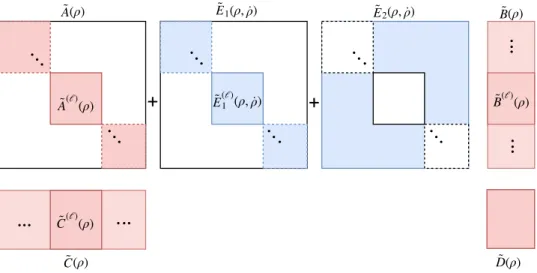
AssumeM clusters have been generated. By rearranging the statex¯ of (8) according to these clusters the obtained system structure is illustrated in Fig. 1. If the new state vector is denoted byx˜ andΠis the permutation matrix mappingx˜tox¯, i.e.x¯= Π˜x, then

A(ρ)˜ = Π^TA(ρ)Π,¯ B(ρ) = Π˜ ^TB(ρ)¯ E(ρ,˜ ρ)˙ = Π^TE(ρ,¯ ρ)Π˙

C(ρ)˜ = ¯C(ρ)Π, D(ρ) =˜ D(ρ)

(10)

Without E(ρ,^˜ ρ)˙ the dynamics are fully decoupled into M subsystems G^˜(`)(ρ) = h _˜

A^{(`)</sup>(ρ) ˜B<sup>(`)}(ρ) C˜^{(`)</sup>(ρ) D<sup>(`)}(ρ)

i

, `= 1, . . . , M. The dimension of each subsystem equals to the size of the corresponding cluster. If we have decided earlier to neglect the coupling term E(ρ,<sup>˜</sup> ρ)˙ , then these subsystems can be handled separately. Otherwise, the coupling term has to be taken into consideration. Since a decoupled structure is needed to continue our algorithm, this is only partially possible. For this, letE(ρ,<sup>˜</sup> ρ)˙ be expressed as a sum ofE<sup>˜</sup><sub>1</sub>(ρ,ρ)˙ andE<sup>˜</sup><sub>2</sub>(ρ,ρ)˙ such that the structure of E<sup>˜</sup><sub>1</sub>(ρ,ρ)˙ is aligned with the structure of A<sup>˜</sup> (see Fig. 1). Assuming that the effect of E<sup>˜</sup><sub>2</sub>(ρ,ρ)˙ on the input-output behavior is negligible, we can proceed the computations with the subsystems defined by the system matricesA<sup>˜(`)</sup>(ρ) + ˜E₁^{(`)</sup>(ρ,ρ)˙ ,B<sup>˜(`)}(ρ),C^{˜(`)</sup>(ρ)andD<sup>(`)}(ρ). These systems are also independent, so they can be separately reduced. The neglected term can be treated as a modeling uncertainty during the analysis or control synthesis procedures performed on the reduced order model.^k

kTo further minimize the approximation error, it is a reasonable idea to complete the distance metric (5) with an additional term penalizing large entries inE^˜2(ρ,ρ)˙.

(ρ)

à ^(ℓ) B̃ ^(ℓ)(ρ)

(ρ) C̃ ^(ℓ)

(ρ) D̃

+ +

(ρ, )

Ẽ ₁ ρ˙ Ẽ ₂(ρ, )ρ˙

(ρ, ) Ẽ ^(ℓ)₁ ρ˙ (ρ)

à B(ρ)̃

(ρ) C̃

Figure 1. The structure of the system matrices after clustering:A(ρ) =^˜ blockdiag( ˜A⁽¹⁾(ρ), . . . ,A˜^(M)(ρ)), E(ρ,˜ ρ)˙ is decomposed such thatE(ρ,^˜ ρ) = ˜˙ E1(ρ,ρ) + ˜˙ E2(ρ,ρ)˙ such that the structure ofE^˜1(ρ,ρ)˙ is aligned

with the structure ofA(ρ)^˜ . The white areas denote the zero entries.

4.2. Balanced reduction

Balanced reduction is a fundamental approach for the model reduction of linear (time invariant and varying, as well as parameter-dependent) systems [10], [9]. The key concept is the balanced realization which reveals the controllability and observability properties of the system. After clustering the dynamical modes,M separate LPV systems are obtained, each of which can be given in the following general form:

˙

x^{(`)</sup>= ˜A<sup>(`)}( ˜ρ)˜x^{(`)</sup>+B<sup>(`)}( ˜ρ)u

y^{(`)</sup>= ˜C<sup>(`)}( ˜ρ)x^{(`)</sup>+D<sup>(`)}( ˜ρ)u, (11) where A^{˜(`)</sup>( ˜ρ) = ˜A<sup>(`)}(ρ) + ˜E1(ρ,ρ)˙ and ρ˜= [ρ,ρ]˙. The similarity transformation T( ˜^ˆ ρ), which transforms (11) into balanced form is obtained from the observability Xo^{(`)</sup>( ˜ρ)and controllability Xc<sup>(`)}( ˜ρ) Gramians^∗∗. If the LPV system is given in a state-space form and the structure of the Gramians is a-priori fixed (e.g. in the formXo^{(`)</sup>( ˜ρ) =X<sub>o,0</sub><sup>(`)}+Pnb

i=1X_o,i^{(`)</sup>f<sub>i</sub>( ˜ρ)X<sub>o,i</sub><sup>(`)}andXc^{(`)</sup>( ˜ρ) = X<sub>c,0</sub><sup>(`)}+Pn_b

i=1X_c,i^{(`)</sup>gi( ˜ρ)X<sub>c,i</sub><sup>(`)} where fi( ˜ρ), gi( ˜ρ) are fixed basis functions and X_o,i^{(`)</sup>, X<sub>c,i</sub><sup>(`)}, i= 1, . . . n_b are free variables), thenXo^{(`)</sup>( ˜ρ)andXc<sup>(`)}( ˜ρ)can be obtained as a result of the following optimization problem [9]:

min

X_o,i^{(`)</sup>,X<sub>c,i</sub><sup>(`)},i=1...n_b

X

k

traceX_o^{(`)</sup>( ˜ρk)X<sub>c</sub><sup>(`)}( ˜ρk)

X˙_o^{(`)</sup>( ˜ρk,ν˜s) +A<sup>(`)}( ˜ρk)^TX_o^{(`)</sup>( ˜ρk) +X<sub>o</sub><sup>(`)}( ˜ρk)A^{(`)</sup>( ˜ρk) +C<sup>(`)}( ˜ρk)^TC^(`)( ˜ρk)≺0

−X˙_c^{(`)</sup>( ˜ρk,ν˜s) +A<sup>(`)}( ˜ρk)X_c^{(`)</sup>( ˜ρk) +X<sub>c</sub><sup>(`)}( ˜ρk)A^{(`)</sup>( ˜ρk)<sup>T</sup>+B<sup>(`)}( ˜ρk)B^{(`)</sup>( ˜ρk)<sup>T</sup> ≺0 X<sub>o</sub><sup>(`)}( ˜ρ_k)0, X_c^(`)( ˜ρ_k)0,∀ρ˜_k ∈Θ˜ and∀˜ν_s∈Ω˜

(12)

whereΘ^˜ andΩ^˜ are suitably dense grids overΘ×ΩandΩ×Φ, respectively. This is a nonconvex optimization problem, but if eitherXo^{(`)</sup>( ˜ρk)orXc<sup>(`)}( ˜ρk)is fixed, then the cost function becomes

∗∗The presented balanced reduction algorithm can only be applied to quadratically stable LPV systems. The extension of the method to unstable systems is well documented in [9] and [10]. If the unstable and mixed stability modes are previously identified and separated in the modal form (see Section 3.5), then only the stable part of the system has to be reduced, so the algorithm above can be applied.

linear in the remaining variables, hence the problem reduces to a linear optimization problem with (LMI) constraints. As suggested in the literature by alternately fixing Xo^{(`)</sup>( ˜ρ<sub>k</sub>) and Xc<sup>(`)}( ˜ρ_k) a numerically tractable iterative algorithm is obtained, where an initialXo^{(`)</sup>( ˜ρ<sub>k</sub>)(orXc<sup>(`)}( ˜ρ_k)) can be calculated from the frozen parameter solutions.

Although the above modifications ease the computational burden, the approach still suffers from the curse of dimensionality. The number of decision variables involved, and hence the numerical complexity grows with the state-dimension of the system. If the number of states goes over 30-40, the LMI optimization problem becomes intractable by the currently available semidefinite solvers.

The decomposition of the system into smaller, independent subsystems, offers a remedy for this problem.

Having determined the observability and controllability gramians of every subsystem, the balancingT^{ˆ(`)</sup>( ˜ρ)transformations and the corresponding parameter dependent, generalized singular value trajectories can be determined. The details of the related numerical algorithms can be found in [9]. Applying the balancing transformations on the subsystems the states corresponding to small singular values can be then eliminated. Since theT<sup>ˆ(`)}( ˜ρ)transformations depend on ρand ρ˙, the reduced systems explicitly depend onρ˙andρ¨as well [9].^††

Having reduced the subsystems individually, the reduced dynamics are finally joined together to obtain the low dimensional approximation of (2). To formally express the result, let the balanced state vector of the `-th subsystem be denoted by xˆ<sup>(`)</sup> and let T^ˆ(`)( ˜ρ) be defined such that

˜

x^{(`)</sup>= ˆT<sup>(`)}( ˜ρ)ˆx^(`). Then, by definition the statez of the reduced order model can be computed asz= ˆΠ^TT⁻¹( ˜ρ)˜x, whereT^ˆ( ˜ρ) =blockdiag( ˆT⁽¹⁾( ˜ρ), . . . ,Tˆ^(M)( ˜ρ)),

Π =ˆ blockdiag( ˆΠ⁽¹⁾, . . . ,Πˆ^(M)) Πˆ^{(`)</sup>= [<sup>I</sup>dim(z<sup>(`)}) 0]^T, such thatz^(`)=

Πˆ^(`)T

ˆ x^(`),

and z<sup>(`)</sup>denotes the state of the `-th reduced subsystem. DefineW( ˜ρ) = ˆΠ^TTˆ⁻¹( ˜ρ)andV( ˜ρ) = Tˆ( ˜ρ) ˆΠ. Then the reduced order model can be expressed as follows:

˙

z= W( ˜ρ) ˜A( ˜ρ)V( ˜ρ)−W( ˜ρ) ˙V( ˜ρ) +W( ˜ρ) ˜E2( ˜ρ)V( ˜ρ)

z+W( ˜ρ) ˜Bu

y= ˜C( ˜ρ)V( ˜ρ)z+ ˜D( ˜ρ)u (13)

Since termE^˜₂has been neglected in the reduction procedure, the termW( ˜ρ) ˜E₂( ˜ρ)V( ˜ρ)appears in the reduced order model. This term can be considered as an additive uncertainty that has to be taken into consideration during the model based control synthesis.

5. CASE STUDIES 5.1. A benchmark example

As a first example a 80 dimensional, 2-input-2-output LPV system has been generated for the numerical evaluation of the developed algorithm. The procedure used to generate the model consists of 4 steps. First, the parameter-variation of each eigenvalue is defined over the parameter domain Ω = [0,1]. The obtainedλ_i(ρ)functions are then used for constructing a parameter-varying block- diagonalA0(ρ)∈R^80×80matrix. This is then completed with a randomly generated constant input B0∈R^80×2 and output C0∈R^2×80 mappings, as well as a constant direct feedthrough term D0∈R^2×2. To make the problem more realistic and industrially relevant, the generated modal system is transformed in the second step by a parameter-varying matrixT(ρ).T(ρ)is constructed by randomly generating an invertible matrix and making its certain (randomly selected) blocks

††If the second derivative ofρis not bounded or its bounds are unknown, then by simply removing theρ˙-dependence of the Gramians also eliminates the explicitρ¨-dependence of the reduced order system.

−7 −6 −5 −4 −3 −2 −1 0 1 2

−2

−1.5

−1

−0.5 0 0.5 1 1.5 2

Real

Imaginary

0.2 0.4 0.6 0.8 1

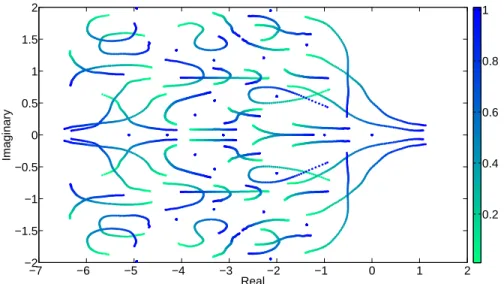
Figure 2. Pole migration of the LPV benchmark system. The value of the scheduling parameter is indicated by colors according to the color-bar on the right.

parameter-dependent. The resulting LPV system can be given as follows:

G0(ρ) :

x˙ =T(ρ)⁻¹A0(ρ)T(ρ)x+T(ρ)⁻¹B0u

y=C0T(ρ)x+D0u (14)

The third step is evaluating the system over an equidistant gridΓ0containingN0parameter values.

Then ad-th degree polynomial is fitted to each entry of the system matrices in order to deform the eigenvalue trajectories and thus make the model more realistic. Finally, in the fourth step, a grid- based representation is generated by evaluating the model over the gridΓ. This way, the LPV system is free from any special structure and can be considered as a generic parameter-varying model. To obtain the particular model used in this section the lengthN₀ of the initial grid, the lengthN of the final grid and the degreedof the interpolating polynomials have been chosen to be60,100and 14, respectively. Furthermore, to evaluate and challenge the algorithm, a wide range of dynamical behaviors have been covered including:

• parameter varying real- and complex conjugate eigenvalues,

• parameter independent dynamics,

• higher order complex and real eigenvalues (with algebraic multiplicity),

• integrators,

• mixed stability eigenvalues (that cross the imaginary axis),

• complex conjugate - real transitions.

These modes can be recognized on the eigenvalue trajectories depicted in Figure 2. The numerical testing of the algorithm can be performed according to the following steps:

• Eigen-decomposition. Using standard numerical methods, the eigenvalues and the corresponding eigenvectors of theA_kmatrices are computed at each grid point.

• Identification of integrators. An initial ordering is carried out, based on the absolute value of the eigenvalues in order to locate and label integrators for further computations.

The eigenvalues corresponding to the integrators are simply removed from the reduction procedure, and will be added back later, before applying the Procrustes algorithm to smooth the eigenvectors.

• Finding the eigenvalue trajectories.The samples of the pointwise modes over the parameter domain are connected by the Hungarian Algorithm, based on their weighted hyperbolic

distance. Unstable poles are projected into the unit circle during the construction of the distance matrix, as discussed in APPENDIX A. Continuous eigenvalue trajectories are restored as a function of the scheduling parameter. Integrators are excluded from the pairing and matched individually.

• Detection of multiple eigenvalue trajectories. Eigenvalue trajectories which are in close proximity for every value of the scheduling parameter are grouped together and handled as muliple ones. In a same manner, using the hyperbolic metric between trajectories, irregular behaviours (i.e. complex-real transitions) can be detected and labelled. For example, in this particular example there are two eigenvalues very close to each other, accompanied by occasional complex-real transitions. This represents discontinuity in the eigenspace (assumptions (A) and (B) are violated), hence a numerical correction was necessary. The absolute variance for the corresponding poles over the scheduling parameter domain was found to be in the range of10⁻⁷ clearly indicating a constant real pole with multiplicity of 2. Therefore we can replace the values with their average, and the complex eigenvectors can be replaced by the closest real eigenvectors. These steps succesfully resolve the mathematical discontinuity without effecting the input-output behaviour.

• Eigenvector smoothing. The complex Procrustes problem is solved for the matched eigenvectors, where the subspaces of the previously labelled poles are treated accordingly.

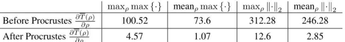
The smoothness of the modal transformations are analyzed numerically, by comparing theρ˙ dependent terms. For this purpose, a cubic spline interpolation is applied for the eigenvectors obtained from the eigen-decomposition, and for the one obtained through the Procrustes problem. These continuous functions are then evaluated between grid points. The results are summarized in Table I, where the large entries indicate discontinuity in∂T¯(ρ)/∂ρ, which implies that the state transformationT^¯(ρ)is probably not differentiable. The results illustrate the effectiveness of the proposed complex Procrustes smoothing.

max_ρmax{·} meanρmax{·} max_ρk·k₂ meanρk·k₂ Before Procrustes^∂T_∂ρ^(ρ) 100.52 73.6 312.28 246.28

After Procrustes ^∂T_∂ρ^(ρ) 4.57 1.07 12.6 2.85

Table I. Numerical comparison of the maximal elements and the matrix norms of modal transformations before- and after smoothing, over the parameter domain. The numerical values were obtained by applying the functions labelling the columns to the matrices labelling the rows, i.e. the 1,1 entry is obtained by

computing the maximal entry of∂T¯(ρ)/∂ρas a function of the parameter and maximizing it overρ.

• Modal form.Applying transformationT^¯(ρ), the parameter-varying modal form is obtained.

At this point a numerical test was carried out to investigate the effect of the ρ˙-dependent term. In this particular example this term can be neglected without significant change in the input/output response. (see also Table I).

• Stable-unstable decomposition. By using the continuous eigenvalue trajectories and the parameter-varying modal form, unstable (as well as mixed stability) dynamics can be separated and removed from the system. In the underlying example, five states were separated (see Figure 2) and thus the model reduction is performed for the remaining 75 (stable) states.

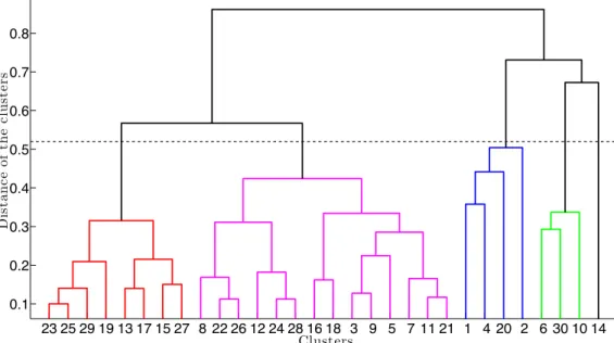
• Clustering.Hiearchical clustering of the matched eigenvalue trajectories are performed next, aiming to reveal dynamical redundancies of the system. Figure 3 shows the corresponding dendrogram plot, which is used for representing the arrangement of the clusters. In Figure 3 the height of each line equals to the distance between the two data objects (either eigenvalue trajectory or cluster of trajectories, computed by (9) ) below. Based on the dendrogram, different number of clusters can be generated and it is the task of the user to decide. To make this decision the following trade-off has to be taken into consideration: large number of clusters corresponds to smaller sized groups, in which state elimination is generally more conservative (consider the extreme case, where each cluster contains a single mode). On the other hand, small number of clusters imply higher dimensional groups with increasing numerical burden (on the other extreme: the entire system considered as a single cluster).

Taking this into account, the given system are subdivided into five clusters (see Figure 3), with the following dimensions: 26 (red), 34 (purple), 7 (blue), 6 (green) and 2 (black). Note that the last cluster cannot be reduced, since it contains a single complex-conjugate mode.

According to Figure 3, a dynamic dissimilarity can be observed, implying the preservation of this mode in question.

23 25 29 19 13 17 15 27 8 22 26 12 24 28 16 18 3 9 5 7 11 21 1 4 20 2 6 30 10 14 0.1

0.2 0.3 0.4 0.5 0.6 0.7 0.8

Clusters

Distanceoftheclusters

Figure 3. Dendrogram for clustering in the benchmark example. The horizontal axis is labelled by the indices of the data objects (eigenvalue trajectories) while the vertical axis shows the similarity distance computed by using (9). The dashed line indicates the threshold where the dendrogram was cut to obtain the 5 clusters.

In addition, the cophenetic correlation coefficient is computed, which is often used for characterizing a dendrogram: how faithfully does it represent the similarities among data objects [40]. The magnitude of the cophenetic correlation should be close to1for the case of a good description. The computed value was0.83, which shows that the selected hyperbolic metric is indeed a good indicator for comparing different dynamical behaviours.

• Computing Gramians.The parameter-dependent controllability and observability Gramians are computed for each individual cluster. By fixing the structures of the Gramians as Xc^{(`)</sup>(ρ) =X<sub>c,0</sub><sup>(`)}+ρX_c,1^{(`)</sup>andXo<sup>(`)}(ρ) =X_o,0^{(`)</sup>+ρX<sub>o,1</sub><sup>(`)}the iterative optimization (Section 4.2) is carried out for each sub-system by using the MOSEK optimization tool [42]. This corresponds to (351 + 595 + 28 + 21)×4 decision variables in four separate optimization problems, which is a significant decrease compared to the5550×4variables involved in the single LMI problem for the entire75dimensional system.

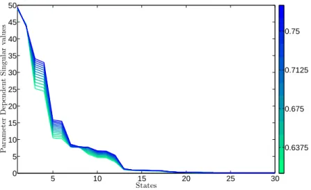
• Singular Value Decomposition.In order to determine the number of states with the largest contributions to the input-output behaviour of each subsystem, the parameter-varying generalized singular values are computed for the subsystems by [9] The number of most significant singular values followed by the dimension of the corresponding cluster are5/26, 5/34,3/7and2/6.

• Balanced Transformation. The parameter-varying balancing transformations and their inverses can be computed for each subsystem, using the singular value decomposition [9].

Applying these transformations, balanced forms are obtained, resulting in aρ,ρ˙ dependent system. The balanced models are then truncated according to the most significant singular values, computed in the previous step. That is, the75dimensional stable part is reduced to17 dimension.

• Reduced model construction.Finally, the individually reduced subsystems are joined together and the five dimensional unstable dynamics are added back. Hence the final, reduced-order

0 0.1 0.2 0.3 0.4 0.5 0.6 0.7 0.8 0.9 1 0

0.1 0.2 0.3 0.4 0.5 0.6 0.7 0.8 0.9 1

Scheduling parameter

ν-gapmetric

Figure 4.ν-gap metric of the full (80) and reduced (22) order model over the scheduling parameter domain LPV model has22 states (compared to the original80) and given in a grid-based fashion, depending onρandρ˙.

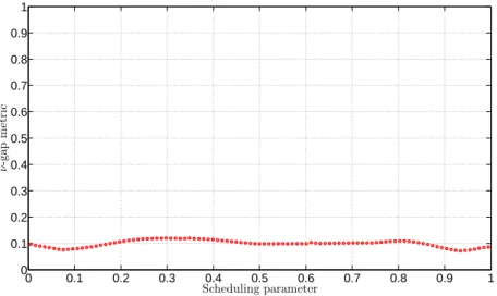
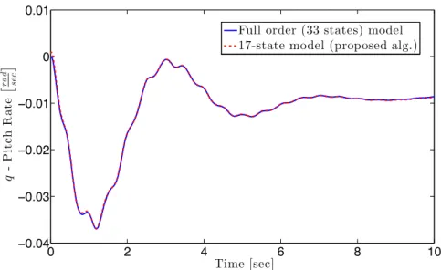
• Evaluation of the reduced model.In order to validate the reduced model, various numerical properties have been investigated. One of the main motivation of model reduction is to obtain a smaller dimensional representation, which is suitable for controller design. From this point of view, similartity of closed-loop behaviours between the high-order and low-order models is of capital importance. In order to take the feedback control objective into account, the widely- usedν-gap metric is evaluated, defined between LTI systems,G₁(jω)andG₂(jω), as [43], [44]:

δν(G1(jω), G2(jω)) =

^(I+G2(jω)G

∗

2(jω))⁻¹²(G₁(jω)−G₂(jω))(I+G^∗₁(jω)G₁(jω))⁻¹² ∞

. (15) Essentially, ifδν(G1, G2)≤β, then a controller, which stabilizesG2also stabilizesG1, with a stability margin ofβ[44]. For identical systemsδν(G1, G2) = 0, otherwise it is0≤δν ≤1. For LPV systems (15) can be interpreted in different ways. One possibility is to compare point-wise LTI systems of the LPV dynamics by taking:

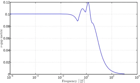
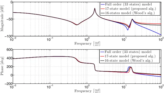
maxω δν(Gk(jω),G˜k(jω)) (16) at each grid point k∈[1 100]. Figure 4 shows the evaluation of the above expression for models interpolated between the original grid points. The maximal value is0.12, implying a satisfactory similarity between the full and reduced order models. The second representation of (15) is illustrated on Figure 5, where the interpolated systems are compared at everyωi

frequency, i.e.:

maxρ δν(G(ρ)(jωi),G(ρ)(jω˜ i)). (17) Figure 5 also provides an insight on the frequency-domain properties of the LPV model reduction.

Finally, the proposed algorithm is compared with a local reduction approach. At each grid point a balanced transformation based model reduction is performed for the corresponding high dimensional LTI model. The local Hankel singular values imply lower dimensional models, within the range of 2−10, for the sake of consistency the dimension has been

100⁻⁶ 10⁻⁴ 10⁻² 10⁰ 10² 10⁴ 0.02

0.04 0.06 0.08 0.1 0.12

Frequency#rad sec

$

ν-gapmetric

Figure 5. Frequency-wise maximumν-gap metric of the full (80) and reduced (22) order model over the scheduling parameter domain

−8 −6 −4 −2 0 2

−2.5

−2

−1.5

−1

−0.5 0 0.5 1 1.5 2 2.5

Real

Imaginary

−8 −6 −4 −2 0 2

−2.5

−2

−1.5

−1

−0.5 0 0.5 1 1.5 2 2.5

Real

Imaginary

0.2 0.4 0.6 0.8 1

Figure 6. Pole migration map for the reduced order model (left) and for the collection of locally reduced systems (right). The value of the scheduling parameter is indicated by colors according to the color-bar on

the right.

fixed for 10 at each grid-point. This fact indicates some conservativeness of the proposed methodology, which, in general preserves more states as a consequence of the modal decomposition. The pole migration maps for the two approaches are compared in Figure 6. It can be observed, that the resulting parameter varying model has a smooth pole map, which makes the LPV model generation straightforward and less challenging. On the other hand, the pole map for the set of locally reduced models shows large variation (see the right plot in Figure 6). This implies the need of a more refined interpolation technique to successfully recover time domain behaviour of the original plant, which also makes control design virtually infeasible.

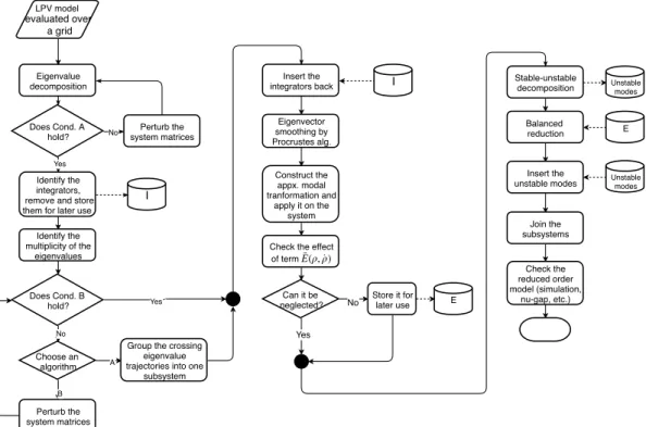
The complete flowchart representing the model reduction workflow is presented in Fig. 7.