Complexity of 2D bootstrap percolation difficulty: Algorithm and NP-hardness
Ivailo Hartarsky
∗Tamás Róbert Mezei
†September 23, 2020
Abstract
Bootstrap percolation is a class of cellular automata with random initial state. Two-dimensional bootstrap percolation models have three rough universality classes, the most studied being the “critical” one.
For this class the scaling of the quantity of greatest interest (the critical probability) was determined by Bollobás, Duminil-Copin, Morris and Smith [5] in terms of a simply defined combinatorial quantity called
“difficulty”, so the subject seemed closed up to finding sharper results.
However, the computation of the difficulty was never considered. In this paper we provide the first algorithm to determine this quantity, which is, surprisingly, not as easy as the definition leads to thinking.
The proof also provides some explicit upper bounds, which are of use for bootstrap percolation. On the other hand, we also prove the negative result that computing the difficulty of a critical model is NP-hard. This two-dimensional picture contrasts with an upcoming result of Balister, Bollobás, Morris and Smith [3] on uncomputability in higher dimensions.
The proof of NP-hardness is achieved by a technical reduction to the Set Cover problem.
MSC2010: Primary 68Q17; Secondary 03D15, 60C05
Keywords: bootstrap percolation, critical models, difficulty, complexity, NP-hard, decidable.
∗DMA, CNRS, UMR 8553, École Normale Supérieure, PSL University, Paris.
Present address: CEREMADE, CNRS, UMR 7534, Université Paris-Dauphine, PSL University, Place du Maréchal de Lattre de Tassigny, 75016, Paris, France. The author was supported in part by European Research Council Starting Grant 680275 MALIG.
hartarsky@ceremade.dauphine.fr
†Alfréd Rényi Institute of Mathematics, 13–15 Reáltanoda utca, 1053 Budapest, Hungary.
The author was supported in part by the National Research, Development and Innovation Office (NKFIH) grant K-116769 and KH-126853.
mezei.tamas.robert@renyi.hu
1 Introduction
1.1 Background
Bootstrap percolation is a class of cellular automata whose first representative was introduced in 1979 by Chalupa, Leath and Reich [7] in statistical physics.
Further applications to several other areas have been considered, namely dynamics of the Ising model, kinetically constrained models for the glass transition, abelian sandpiles and others (see a recent review of Morris [18] for more information).
We consider the following iterative discrete-time process on the elements (sites) ofZd. At each time t∈N every site is either infected or healthy. We encode the state of all sites by specifying the set of infected sites At. Given a setA⊆Zdor (Z/nZ)d of initially infected sites, more sites become infected at each discrete time step following a deterministic monotone local rule invariant in time and space, while infections never heal. More precisely, let us introduce the broadest framework brought forward by Bollobás, Smith and Uzzell [6].1 A bootstrap percolation model is specified by a finite set U, called the update family, of finite subsets ofZd\ {0}, called rules. For an initial set of infected sites A=A0 ⊆Zd we recursively define for all t∈N
At+1 =At∪ {x∈Zd : ∃U ∈ U, x+U ⊆At}
and [A] =S
t>0At is the closure of A with respect to this operation.
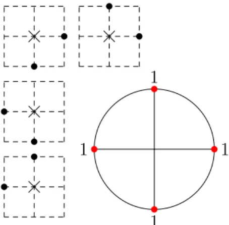
For concreteness, four examples of such models with different update families U are given in Figure 1. We will use those to also illustrate further definitions. For instance, in the East model (see Figure 1a) one infects sites whose bottom or left neighbour is infected, while in the North-East model (Figure 1d) one only infects sites such that both their bottom and left neighbours are infected.
We will only discuss the most studied case, where A is chosen at random according to the product Bernoulli measure Pp, so that each site is initially infected with probability p∈[0,1]. Equipped with this measure, the model exhibits a phase transition at
pc= inf{p∈[0,1] : Pp(0∈[A]) = 1}.
The model is defined identically on tori(Z/nZ)d by setting pc(n) = inf{p∈[0,1] : Pp([A] = (Z/nZ)d)>1/2}.
1Earlier partly non-rigorous considerations of a more restricted class of models can be found in the works of Gravner and Griffeath [10, 11] from the 1990s.
∞
(a) The East model, which is super- critical (with difficulty0).
1 1
1
1
(b) The modified 2-neighbour model, which is critical with difficulty1.
1 2
∞
(c) A toy model, which is critical with difficulty 1.
∞
(d) The North-East model, which is subcritical (with difficulty ∞).
Figure 1: Four example bootstrap percolation models. For each one the rules are depicted on the left with 0 marked by a cross, the sites of each rule denoted by dots and the grid lines dashed. The figure on the right gives the stable directions in red with their difficulties next to them. The isolated stable directions are marked by red dots.
In this background section we consider n →0and use associated asymptotic notation. Namely, given a function f(n) we write O(f(n)) for a function bounded in absolute value by Cf(n) for some constant C not depending on n (but possibly depending on U). We write Θ(f(n)) for a function that is bounded above by Cf(n) and below by cf(n) for some positive constants c and C, neither depending on n. We will use analogous notation in later sections with respect to other diverging parameters.
Although for some concrete models higher dimensions have been un- derstood and some general universality conjectures have been put forward in [2, Conjecture 16] and [5, Conjecture 9.2], we will restrict our attention to the 2-dimensional case. The results of Bollobás, Smith and Uzzell [6]
and Balister, Bollobás, Przykucki and Smith [2] combined establish that all bootstrap percolation models can be partitioned (by a simple procedure) into 3“rough universality classes” with qualitatively different scaling of pc(n). In order to define these we need some notation. For a direction u in the unit circle S1 ={x∈R2 : kxk2 = 1}, which we standardly identify with R/2πZ, we denote by
Hu ={x∈Z2 : hx, ui<0}
the open half-plane with normal u and by
lu ={x∈Z2, hx, ui= 0}
the line passing through 0 perpendicular to u. A direction u is unstable if there exists U ∈ U such that U ⊂Hu and stable otherwise. It is not difficult to show that the unstable directions form a finite union of open intervals in S1 with rational endpoints, that is a direction u such that lu∩Z2 6= ∅. Indeed, each rule individually induces a (possibly empty) interval of unstable directions with endpoints perpendicular to sites in the rule (so in Z2), there are finitely many rules and, by definition, the union of these intervals is the set of unstable directions for the full model. Thus, the set of stable directions is a finite union of closed intervals with rational endpoints in S1, some of which may be reduced to a single point called isolated stable direction.
As an example, let us consider the modified2-neighbour model (Figure 1b).
The top-left rule consisting of(1,0) ∈Z2and(0,−1) ∈Z2makes all directions in the open interval (π/2, π)⊂S1 unstable. By invariance by rotation by π/2 there remain only the four isolated stable directions shown in Figure 1b. The reader is encouraged to check the stable directions of the other examples in Figure 1.
We are now ready to define the partition into rough universality classes conjectured in [6] and proved in [2, 6] is in terms of these directions.
• U issupercritical if there exists an open semi-circle of unstable directions, in which case pc(n) = n−Θ(1).
• U is critical if it is not supercritical and there exists a semi-circle with a finite number of stable directions, in which case pc(n) = (logn)−Θ(1).
• U is subcritical otherwise (if each semi-circle contains infinitely many stable directions), in which case pc >0.
Let us check that the modified 2-neighbour model (Figure 1b) is critical. As observed before, the only stable directions are the four axis directions. In particular, every open semi-circle contains either one or two of them. For the toy model (Figure 1c) again every open semi-circle contains at least one of the stable directions, but e.g. the semi-circle (−π/2, π/2)⊂S1 only contains one stable direction, so it is also critical. For the East model the same semi-circle contains no stable directions, making it supercritical. Finally, in the North-East model there is only a single quarter of a circle of unstable directions. In particular, every half-circle contains infinitely many unstable directions, so the model is subcritical.
The behavior of supercritical models is dominated by the study of finite infected sets with infinite closure (a single infected site in the East model), while subcritical ones are more closely related to percolation (for example, the North-East model is equivalent to classical oriented site percolation if one considers healthy sites). The most studied models are critical ones, to which the archetypal example of bootstrap percolation belongs — the 2-neighbor model, in which a site becomes infected if at least two of its nearest neighbors are already infected. Note that the modified 2-neighbour model in Figure 1b does not infect a site if it only has2infected neighbours which are on opposite sides of it, however, from the point of view of stable directions and difficulties to be defined later, this modification is of no importance. The 2-neighbour model is the first one for which the rough universality result above (and more) was established — by Aizenman and Lebowitz [1]. They realized that the dynamics is dominated by a bottleneck — creating an infected “droplet”
of a certain “critical” size, which can then easily grow out to infinity, and proved that for this modelpc(n) = Θ(1/logn). In a substantial breakthrough Holroyd [16] determined the asymptotic location of the sharp threshold and since then much sharper results have been proved [12, 15]:
pc= π2
18 logn − Θ(1) (logn)3/2.
Such sharp or sharper bounds have been obtained for a handful of other specific models [4, 8, 9], but still remain open in general. However, the level of
precision of the Aizenman-Lebowitz result was established in full generality for critical models by Bollobás, Duminil-Copin, Morris and Smith [5]. They introduce the following key notion of difficulty.
Definition 1.1 (Definition 1.2 of [5]). LetU be a critical model and u be a direction. If u is an isolated stable direction, we define its difficulty,α(u), to be the minimum cardinality of a setZ ⊆Z2\Hu such thatZ¯ := [Hu∪Z]\Hu
is infinite. For unstable directions u we set α(u) = 0 and for non-isolated stable ones we set α(u) =∞. The difficulty of U is
α = inf
C∈Csup
u∈C
α(u), (1)
whereC is the set of open semi-circles ofS1.
Let us note that the definition we give is formally different from the one in [5], but it turns out to be equivalent. Indeed, any unstable direction u satisfies [Hu] = Z2, since one can infect 0by definition of unstable directions and, by translation invariance one can infect lu, so that a translate of Hu
becomes infected and one may conclude by induction. Here we used that for any rational direction, we can write Z2 =F
i∈Z(lu+i·xu) for some vector xu ∈Z2, where we write A+x for{a+x, a∈A}for any set A ⊆Z2 and site x∈Z2. For stable directions the equivalence is proved in Lemma 2.7 of [5].
For the reader’s convenience, let us determine the difficulties of the stable directions of the toy model of Figure 1c. By definition unstable directions have difficulty 0 and non-isolated stable ones have difficulty ∞, so we are left with the right (0) and top (π/2) isolated stable directions. Let us start with the direction 0. Since it is stable[H0] =H0, we haveα >1.2 However, [H0 ∪ {(0,0)}] = H0 ∪l0, since one can infect (0,−1) by the second rule (see Figure 1c) and, inductively (0,−k) for all k ∈N; one can also use the first rule to infect (0,1)and then (0, k)for all k ∈Nonce (0,0)and (0,−1) are infected. No further infections occur, as u is stable and Hu ∪lu is a translate of Hu. Thus, α(0) = 1, as l0 ={(0,0)} is infinite (lu is infinite for any rational direction u). Turning to u =π/2, we have α(u)>1 as before, and one can check as above that [Hu ∪ {(0,0),(1,0)}] = Hu ∪lu using the first and third rules. It remains to see that there does not exists x∈Z2 such that {x} is infinite, in order to conclude that α(u) = 2. Indeed, all rules contain at least 2sites in Z2\Hu, so for anyx we have[{x} ∪Hu] = {x} ∪Hu. Finally, once we know that α(π/2) = 2 and α(0) = 1, we have that the open half-circle (−π/2, π/2) only contains one stable direction and it has difficulty
2More generally, for any model and any isolated stable directionuwe have16α(u)<∞ (see Lemma 2.7 of [5]).
1, so α 6 1, which is the smallest possible value for a critical model: by definition, every half-circle contains a stable direction and, as we noted, only unstable directions have difficulty 0.
The result of [5] states that3
pc(n) = (log logn)O(1) (logn)1/α .
1.2 Results
So far it has not been investigated how one could determine the difficulty α in practice, mainly owing to the simple definition and to the fact that for simple models such as the ones in Figure 1 this is straightforward. In this paper we consider α from a computational perspective.
Throughout the paper, we assume that U is described as a family of sets of pairs of integer coordinates represented in binary. Therefore the size of the input is proportional to
kU k:= logD·X
U∈U
|U|, (2)
whereD is the “diameter” of U: D= 2·max
(
kxk∞ : x∈ [
U∈U
U )
. (3)
A further justification of the need to takeD into account in kU k is provided in the Appendix showing that the difficulty α is not bounded in terms of P
U∈U|U| only. Our first result is that α is computable. We prove this by giving an explicit algorithm and bounding its complexity.
Theorem 1.2. There exists an algorithm which, given a critical bootstrap percolation update family U, computes its difficulty α.4
Remark 1.3. In fact, it is not hard to check that our algorithm runs in time at most
|U |2·2D2(1+o(1)) = exp(O(D2)),
which is in the worst case at most doubly exponential in kU k. This bound is as sharp as a bound in terms of D only can be. Indeed, |U |=eO(D2) and|U | can be as large as 2D2.
3They actually give matching bounds up to a constant factor, which requires dividing critical models into two subclasses with different logarithmic factors.
4This result is proved independently by Balister, Bollobás, Morris and Smith [3].
Explicit bounds analogous to the ones derived in the proof of Theorem 1.2 are the only missing ingredient causing the constants appearing in the main results of [5, 14] to be implicit (cf [5, Lemma 6.5] and its version in [14]).
Moreover, a corresponding uncomputability result in higher dimensions based on supercritical models in two dimensions has been announced by Balister, Bollobás, Morris and Smith [3] prior to our work. As that could lead one to expect, Theorem 1.2 is not at all automatic.
On a high level, the main idea behind our proof is that if a half-planeHu
is infected, the process restricted to the line lu is a 1-dimensional bootstrap percolation process. Owing to the bounded range of the rules and translation invariance, the final state of this process is either periodic with bounded period or finite, which two possibilities can be distinguished in a correspondingly bounded time.
On the other hand, we also prove the following negative result.
Theorem 1.4.The problem of computing the difficultyαof a critical bootstrap percolation update family U is NP-hard.
This result is proved by a fairly technical reduction to the Set Cover decision problem in Section 3. Besides the result of [3], another reason to expect that the problem of determining α is hard in a sense made clear in Theorem 1.4 is a recent parallel notion of difficulties adapted to subcritical models termed “critical densities”. Those were introduced by the first au- thor [13] and they are clearly far too complicated for one to expect to be able to compute them. From this point of view the result of Theorem 1.4 is not unexpected.
2 Decidability: proof of Theorem 1.2
In this section we provide an algorithm to compute the difficulty of a critical model. Let us stress that it is not optimized and is only meant to prove Theorem 1.2.
Proof of Theorem 1.2. Fix an update family U. To start, let us see how to determine the set of stable directions in time polynomial in the size of the input kU k. Indeed, for each site x in each rule U we determines its polar coordinates (rx, θx) = (kxk2, x/kxk2) ∈ R+×S1. On the practical side, rx can be represented as the square root of an integer bounded by D2 andθx can be encoded by its tangent, which is rational with numerator and denominator bounded by D, and one boolean indicating whether θx ∈(−π/2, π/2). Then for each rule U we take an arbitrary x0 ∈ U and compute θx −θx0 for
all x ∈ U (its tangent is still rational and its numerator and denominator are bounded by D2). We determine the largest and smallest such values, δ+, δ−, considering differences in(−π, π]. Finally, the unstable interval of U is (θx0 +δ++π/2, θx0 −δ−+ 3π/2) ⊂S1 (which is empty if δ+−δ− >π). The set of unstable directions is then the union of these intervals for allU ∈ U. In particular, the isolated stable directions and, more generally, the endpoints of the intervals of stable directions forU are among the endpoints of the intervals for different U, so there are at most 2|U |of them. In order to determine this union in practice it suffices to check for each of these endpoints whether it is stable (not contained in any of the unstable intervals for other U ∈ U) and keep the information whether it was a left or right endpoint of the associated interval. Hence, the preliminary step of determining the (isolated) stable directions is completed in polynomial time inkU k. It is also not hard to verify for each of the |U | right-endpoints whether there exists a stable direction in the half-circle starting there and whether there are finitely many of them (i.e.
all are isolated), which allows one to decide if U is supercritical, critical or subcritical in polynomial time.
Assuming that U is determined to be critical, we can use (1) to compute the difficulty, α, once we know all α(u) ∈ N for isolated stable directions.
Indeed, for each of the open semi-circles with one endpoint among those considered above, we only need to calculate the maximum of α(u)for isolated stable directions u(if there are any non-isolated directions, we do not need to consider the semi-circle). As this can also be done in time polynomial in kU k, we will now fix an isolated stable direction u and provide an algorithm for determining α(u).
We shall assume thatD is sufficiently large throughout the proof. Indeed, given D, all U ∈ U are distinct subsets of {−D/2, . . . , D/2}2, so there are at most 22(D+1)2 possible U and |U | 6 2(D+1)2. Therefore, the algorithm’s asymptotic complexity is only determined by families with large values of D, as one can directly list the difficulties for isolated stable directions with
“small” values of Din constant time.
Recall the notation Z¯ from Definition 1.1, which we shall use without specifying u, as it will be clear from the context. In order to determine α(u) we will use the following lemmas to bound the size of the set Z in Definition 1.1. The first of these is a one-dimensional result which we shall reduce the problem to.
Lemma 2.1. Let U be an update family, let u ∈ S1 be an isolated stable direction and let A be a finite subset of lu. Then the set A¯ is either infinite or its maximal distance from A is at most D3·2D.
Proof. Observe that by stability of u we have A¯ ⊂ lu. Then the dynamics started from Hu∪A can be viewed as a dynamics on lu only. Note that lu consists of integer sites on a line, so it is naturally identified with Z by the composition of a homothety and a rotation. Furthermore, we know that uis an isolated stable direction and, thereby, lu+π/2 (which is simply a rotation of lu) contains a site xin some U ∈ U with kxk∞6D/2 by (3). Hence, the homothety ratio is between 1/D and 1.
Notice that the dynamics restricted to lu is simply a 1-dimensional boot- strap percolation process, where each rule U ∈ U is replaced by U ∩lu if U ⊂ (Hu ∪lu) and removed otherwise. It therefore suffices to prove the following claim, which concludes the proof.
Claim. For a one-dimensional bootstrap percolation family and a finite set A⊂Z, we have that A¯is either infinite or its maximal distance from A is at most D2·2D.
Proof. Denote A={a1, . . . , an}with a1 <· · ·< an. Let us denote byP the property that the following three conditions hold:
• |[A]|<∞,d(s, A)6D·2D+1 for all s∈[A],
• max[A]−an6D·2D+1−D,
• a1 −min[A]6D·2D+1−D.
Let A be minimal with respect to inclusion violating P. We next prove that
|[A]|=∞.
Base. Assume that|A|= 1, without loss of generality A ={0}. If [A] = A, we have nothing to prove, as P clearly holds. Otherwise, assume thatx∈Z becomes infected on the first step. Then, since {0} is the only infected site initially, {x} is a rule in the update family. However, that entails that k.x becomes infected on the k-th iteration at the latest and, in particular, [A]is infinite.
Step. Assume that |A|>1. Assume for a contradiction that there exists 0 < i < n and b ∈ [A] such that ai+1 > b > ai and min(b−ai, ai+1 −b) >
D·2D+1. Then, by minimality of A, bothA0 ={a1, . . . , ai} andA00= A\A0 satisfy P. Therefore,
min[A00]−max[A0]> D·2D+2−2(D·2D+1−D)> D,
so that [A] = [A0]∪[A00], which contradicts the existence of b∈[A]. Indeed, there is no site in Z such that a rule translated by it intersects both[A0]and [A00] and by definition of the closure those do not evolve under the dynamics.
Assume next that max([A]) > an+D·2D+1−D (the corresponding case for min([A])is treated identically). Then, by the pigeon-hole principle, there exist b, c∈Zwith an+D < b < c−D <max([A])−2D such that
∅6= [A]∩[b, b+D−1] = ([A]∩[c, c+D−1])−(c−b)
(since no infection can cross a region of size D not intersecting [A]to reach max([A])). Therefore, [A]∩[b, b+D−1] infects a translate of itself, since the dynamics to the right of b+D is not affected by infections to the left of b, once we fix the state ofb, . . . , b+D−1. Similarly to the case |A|= 1, this is a contradiction with |[A]|<∞, which concludes the proof.
The next lemma is an application of the covering algorithm of [6]. For the sake of completeness, we will include a sketch of it in the proof.
Lemma 2.2. Let U be a critical update family and u be an isolated stable direction. Let Z ⊂Hu+π be a set of size at most D. Then for every z ∈[Z]
we have hz, ui>−O(D4).
Proof. First, we prove the following claim.
Claim. There exists a set T ⊃ {u} of three or four stable directions con- taining the origin in their convex envelope (if viewed as a subset of R2) such that for eachv ∈ T there exists x∈Z2∩vR such thatkxk∞6D/2and such that for every v, w∈ T we have |v−w+π|>2/D2.
Proof. First assume that u+π is unstable. LetT consist of u and the stable directions, u+π+δ+ and u+π−δ− (δ±∈(0, π]), closest to u+π in both semi-circles with endpoint u+π (these exist as the set of stable directions is closed). Furthermore, recalling that U is not supercritical, there is no semi-circle of unstable directions, so δ++δ−< π. This implies that indeedT contains 0 in its convex envelope.
Assume that, on the contrary, u+π is stable. Consider the semi-circle (u, u+π)⊂S1. In it there exists a stable direction (sinceU is not supercritical).
If there are no unstable directions, we pick u− =u+π/2, otherwise, we set u− to be an isolated or semi-isolated stable direction in that semi-circle. We define u+ similarly in the opposite semi-circle. We set T ={u, u+π, u−, u+}.
It is clear that 0 is in the convex envelope of T.
In both cases T consists of directions which are either isolated, semi- isolated or a rotation by π/2of such a direction. Therefore, as in the proof of Lemma 2.1, there exists a site x as in the statement of the claim.
Finally, let us bound the difference between two directions v 6=w such that there existx∈Z2∩vR andy∈Z2∩wR with max(kxk∞,kyk∞)6D/2.
Indeed, det(x, y)∈Z\ {0}, so
|sin(v−w)|= |det(x, y)|
kxk2kyk2 > 2 D2
and therefore |v−w|>2/D2.
We fix a set T as in the claim. We call aT-droplet a polygon with sides perpendicular to the directions inT. SinceT contains0in its convex envelope there exist T-droplets. Since the difference between consecutive directions in T are at most π−2/D2, we can find aT-dropletP with diameter O(D3) containing [−D/2, D/2]2 ⊇S
U∈U U (e.g. a T-droplet circumscribed around a circle with D).
We can then directly apply the covering algorithm of [6] to conclude the proof. Let us outline that algorithm in our setting. We start with a set of translates of P, namely {z+P, z ∈Z}. At each step if two of the current droplets P1, P2 satisfy that there existsx∈Z2 such that(P+x)∩P1 6= ∅and (P +x)∩P2 6=∅, then we replace them by the smallest T-droplet containing
their union. We repeat this as long as possible.
By Lemma 4.6 of [6] (stating that the diameter of the smallest droplet containing two intersecting ones is at most the sum of their respective diame- ters) the sum of diameters of droplets increases by at most diam(P) =O(D3).
Therefore, in the final set of droplets the total diameter is O(D4), as the number of droplets decreases by 1 at each step. Moreover, by Lemma 4.5 of [6] the union of the final droplets contains [Z], so the proof is complete, as each of the output droplets contains at least one site of Z ⊂H−u.
Algorithm. Let us first describe an algorithm to determine α(u) and post- pone its analysis. For each integer k from 1 to D we successively perform the following operations to determine if there exists a set Z of size k as in Definition 1.1. We stop as soon as such a set is found and return the corresponding (minimal) value of k. For each fixed k we start by choosing a set Z0. The first site is 0 and each new one z is picked within distance D11·2D from some of the previous ones and such that
06hz0−z, ui=O(D4) (4)
for some z0 among the previous ones. There are at most DO(1)·2D
D
= 2D2+o(D2) = exp(O(D2))
such choices. For each of them we successively inspect different translations t ∈Z2, such that06ht, ui=O(D5) and
06ht,(−y, x)i< x2+y2, (5) where (−y, x)∈Z2 is such that (x, y)∈uR and x andy are co-prime, in the (total) order given by ht, ui starting from t= 0. Finally, fixZ =Z0+t.
For each Z we run the bootstrap dynamics with initial set of infections Z ∪Hu until it either stops infecting new sites or infects a site s with ksk∞>D13·2D and hs, ui=O(D5). This can be done by checking at each step each site at distance D13 ·2D +D from the origin for each rule and repeating this for 5D time steps. If the dynamics becomes stationary, we continue to the next choice of Z, while otherwise we return|Z| for the value of α(u).
Correctness. We now turn to proving that the algorithm does return an output and it is precisely α(u). The first assertion is easy. Indeed, as uis an isolated stable direction, (by [5, Lemma 2.8]) there exists a rule U ∈ U with
U ⊂Hu∪ {x∈lu,hx, u+π/2i>0},
so that adding D consecutive sites on lu to Hu is enough to infect a half-line of lu, only taking U into account. Thus, we know that α(u) 6 D and the algorithm will eventually check such a configuration when k =D, unless it has returned a smaller value, and infections will propagate to distance D13·2D (and in fact to infinity). Let us then prove that the output is α(u).
Denote bytj the values of t considered by the algorithm, so thatt0 = 0.
Note that by (5) there exists a single t∈Z2 with a given value of ht, ui, so that this scalar product indeed defines a total order on the values of t and we can also extend our notation toj <0 for convenience, though those are not examined by the algorithm. Further define lj :={s∈Z2,hs, ui=htj, ui}
and Zj =Z0+tj for some Z0 considered by the algorithm, so that l0 =lu by abuse of notation.5
5Here we view 0as an element of Z, possible value ofj, while uis an element ofS1. As we will not make reference tolv withv = 0∈S1, we hope that this will not lead to confusion.
Claim. Assume that a set Zi considered by the algorithm is of size k 6 α(u) and such that Z¯j (recall Definition 1.1) is finite for all 0 6 j 6 i.
Then the maximal distance between a site from Z¯i and Zi is at most D5· 2Dmax(0,hti, ui).
Proof. We prove the statement by induction on i ∈ Z. For i < 0, i.e.
hti, ui<0, thenZi ⊂Hu by (4) and there is nothing to prove, sinceZ¯i = ∅– no additional infections take place. Assume the property to hold for all tj with j 6i. We aim prove the same fori+ 1.
Observe that for each0< j 6i+ 1 we have that
Z¯i+1∩lj ⊆( ¯Zi+1−j ∩l0) +ti+1−ti+1−j. (6) Indeed,Zi+1∪Hu ⊆(Zi+1−j∪Hu) +ti+1−ti+1−j, since Zi+1 =Zi+1−j+ti+1− ti+1−j and Hu +ti+1−ti+1−j ⊃Hu. Furthermore, by stability of u we have thatZ¯i+1∩lj =∅ forj > i+ 1. Also, by (6) and the induction hypothesis we have that Z¯i+1\l0 is at distance at mostD5·2Dhti, ui from Zi+1, so we are left with proving that sites in Z¯i+1∩l0 are at distance at most D5·2Dhti+1, ui from Zi+1.
Consider the set
Z0 ={z ∈Z¯i+1∩l0, d(z, Zi+1)6D+D5·2Dhti, ui}.
By the reasoning above we have that Z¯i+1 ∩ l0 = Z0 ∪Z¯0. However, by Lemma 2.1, Z¯0 cannot be at distance more than 2D ·D3 from Z0, as Zi+1\l0
is at distance at least D from all sites inZ¯i+1\Z0. Recalling the definition of Z0, we get thatZ¯i+1 is at distance at mostD+D3·2D+D5·2Dhti, ui and we are done. Indeed, hti+1−ti, ui>1/D, since there exists a site x∈Z2∩uR with kxk∞6D/2and hti+1−ti, xi>0 is an integer.
The claim clearly implies that the algorithm cannot return a value smaller than α(u). In order to conclude, we need to show that whenk =α(u)among the sets examined by the algorithm there will be a set Z such that there exists z ∈Z¯ with kzk∞>D13·2D and therefore the output will beα(u).
Consider a setZ ⊂Z2\Hu as in Definition 1.1 of sizeα(u)(and therefore minimal). Recall that by Lemma 2.2 every z ∈ Z satisfies hz, ui = O(D4) (otherwise Z¯ = [Z] is finite, asU is not supercritical) and, by stability of u, the same holds for Z. Let¯ P = {x ∈ R,∃z ∈ Z,hz, ui = x} and define P¯ similarly for Z. These are discrete subsets of¯ R. Note that by minimality of Z and Lemma 2.2, P ⊂ R cannot have a gap of length larger than O(D4).
Indeed, there exists x∈P¯ such that infinitely many points of Z¯ project to it and those are all in Z¯0 where Z0 are the sites inZ that project tox0 ∈ P such
that there exist n and x0 =x, x1, . . . , xn =x0 in P with |xj+1−xj|= O(D4) and if Z0 6=Z, we obtain a contradiction with the minimality of Z.
Analogously, let P⊥= {x∈R,∃z ∈Z,hz,(u+π/2)i=x} and define P¯⊥ similarly forZ¯. We claim that itsP⊥ cannot have a gap of length larger than O(D10·2D). This time P¯⊥ is necessarily infinite, as only a finite number of points z ∈ Z2 with hz, ui = O(D4) have the same (u+π/2)-projection.
Considering a set Z0 ⊂Z inducing the corresponding distanceO(D10·2D)- connected component of P⊥ and using the claim instead of Lemma 2.2 as in the previous paragraph, we reach a contradiction with the minimality of Z.
Hence, all Z of sizeα(u) as in Definition 1.1 are in fact considered by the algorithm. Since such a Z with infinite Z¯ exists, the algorithm does indeed output α(u).
3 NP-hardness: proof of Theorem 1.4
In this section we prove Theorem 1.4 by providing a reduction from Set Cover to 2D Critical Bootstrap Difficulty. For the Set Cover problem we consider auniverse {1, . . . , N}and a collectionS of subsets of the universe and assume that |S|>4and N >4. The Set Coverproblem asks for determining the minimum cardinality of a subset of S which covers the universe. It is one of the first NP-complete problems described by Karp [17].
We fix an instance
S ={Si : i∈Z,16i6|S|}.
Our goal is to define a critical bootstrap percolation update family whose difficulty α is (up to a simple transformation) the solution to Set Cover. Let the set of rules associated to S be
US ={U0, U1} ∪ {Ui,jk : 16i6|S|, 16k 6|S|2, i, k∈Z, j ∈Si}, where
U0 =
(−k,0),(0,−k) : 16k 6N|S|2 , U1 =
(+k,0),(0,−k) : 16k 6N|S|2
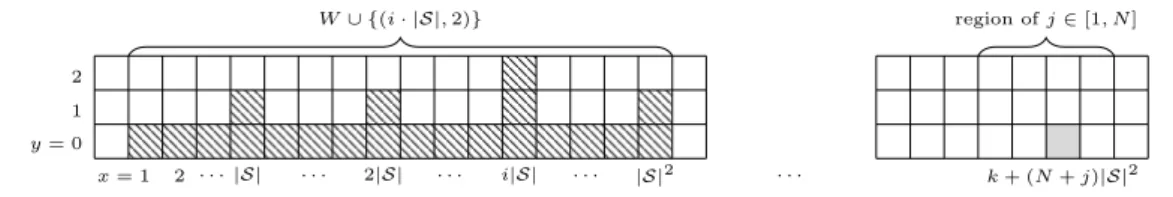
and the rules Ui,jk , defined as follows, share a large portion of their structure (see Figure 2).
T =
(0,−y) : 1 6y6N · |S|2 ,
W ={(x,0) : 16x6|S|2} ∪ {(l· |S|,1) : 16l6|S|}, Ui,jk =T ∪ (W ∪ {(i· |S|,2)})−(k+ (N +j)· |S|2,0)
.
W∪ {(i· |S|,2)} region ofj∈[1, N]
2 . . .|S| . . . 2|S| . . . i|S| . . . |S|2 . . . k+ (N+j)|S|2
x= 1 y= 0
1 2
Figure 2: A visualisation of (Ui,jk \T) + (k+ (N +j)|S|2,0); the shaded cell indicates where the origin is shifted to.
First we claim that the only isolated stable direction is u = π/2 and [−π,0] contains the rest of the stable directions. The unstable intervals corresponding to the rules U0 and U1 are(0, π/2) and(π/2, π), respectively.
The unstable interval ofUi,jk is contained in (0, π/2) for all i, j, k. Thus,US is indeed critical and α(US) = α(u), so that we can focus on this direction.
Let M ⊆ {1, . . . ,|S|} be an optimal solution to the Set Cover problem given by S i.e. a set of minimal size such that
[
i∈M
Si ={1, . . . , N}.
We first claim that, setting
Z0 =W ∪ {(i· |S|,2) : i∈M}
we have [Z0∪Hu]⊃lu, so that
α(u)6|Z0|=|W|+|M|=|S|2+|S|+|M|. (7) Indeed, using once each of the rulesUi,jk for alli∈M,j ∈Si and16k 6|S|2, one infects all sites in
1 + (N + 1)· |S|2,(2N + 1)· |S|2
× {0},
since M is a cover, and those are enough to infect lu using U0 and U1. For any Z ⊆Z2 recall the notationZ¯ = [Z∪Hu]\Hu from Definition 1.1.
To prove that (7) is actually an equality, we suppose that there exists a set Z ⊂Z2 \Hu for which |Z¯|=∞ and |Z|<|Z0|. Fix a minimal such set Z.
First note that|U0\Hu|=N|S|2 and similarly for U1. Therefore, if there exists p∈Z2\Hu such that one of p+U0 and p+U1 is a subset ofZ ∪Hu, then |Z| > N|S|2 > |Z0| – a contradiction. However, in order not to have Z¯ =∅ some of the rules must be applicable to Z∪Hu and therefore there exists p∈Z2 \Hu such that p+W ⊆Z.
Observation 3.1. For anyq ∈Z2\ {0} we have |(q+W)\W|>|S|.
Although the verification is immediate, calling this fact an observation is deceptive, since W is designed to possess this property. It follows that p is unique, otherwise |Z|>|W|+|S|>|Z0| (since any minimal cover is smaller than the universe), a contradiction.
Lemma 3.2. Every point q ∈Z¯\Z has the same y-coordinate as p.
Proof. Suppose that there exists q ∈ Z¯\Z contradicting the statement of the lemma and consider such a q with minimal infection time for the process with initial set of infectionsZ∪Hu. ThenZ contains at least |W| − |S|sites on the row of q, as all rules contain at least as many and by minimality of q.
Therefore,|Z|>2(|W| − |S|)>|Z0|, a contradiction.
By Lemma 3.2 and the fact that(Z∪Hu)−(0,1)⊆(Z−(0,1))∪Hu and (Z∪Hu) + (1,0) = (Z+ (1,0))∪Hu, we can assume without loss of generality
that p= 0.
By the minimality ofZ and Lemma 3.2, the y-coordinate of any site in Z is 0, 1, or 2. Indeed, in order to infect each of the sites q ∈Z¯ ⊆lu, we use one of the rules, but those are all contained in {x∈ Z2,hx, ui 62}, so one can remove any other sites from Z without changing Z¯.
Lemma 3.3. There does not exist q ∈Z2\ {0} such that q+W ⊆Z¯. Proof. Let q be as in the statement of the lemma such that no other q0 +W becomes fully infected before q+W for the process with initial infections Z ∪Hu. By Lemma 3.2 we have thatq ∈lu.
If|x|>|S|2, then by Lemma 3.2 the setZ\W contains at least|W\lu|=
|S| elements (with y-coordinate 1), therefore |Z| > |W| +|S| > |Z0|, a contradiction.
Assume that|x|<|S|2. If lu∩(q+W)\W ⊆Z, then by Observation 3.1 we have |Z| > |W|+|S| – a contradiction. Therefore, some of the sites in lu∩(q+W)\W ⊆Z¯ are infected by the process. However, by minimality of q they can only be infected using U0 or U1. Yet, as soon as one can use rule U0 or U1 to infect a site inlu, the entire lu can be infected using those rules only. Thus, removing from Z every site inZ\W with y-coordinate 1 (and in particular (q+W)\(lu∪W)6=∅) does not prevent the infection of
infinitely many sites, which contradicts the minimality of Z.
By Lemma 3.3 we have that until a ruleU0 or U1 is used the only possible infections are of the form “k+ (N +j)|S|2 becomes infected via rule Ui,jk ”.
Therefore, all sites (x,2) ∈ Z are either redundant (which contradicts the minimality of Z) or satisfy x=i· |S| with 16i6|S|.
Finally, setI ={i : (i· |S|,2)∈Z} and J ={1, . . . , N} \[
i∈I
Si.
Then, in order to have |Z¯| = ∞, it is necessary (and sufficient) to have a sequence of N|S|2 consecutive sites in
(Z ∩lu)∪ {(k+ (N+j)|S|2,0) : i∈I,16k 6|S|2, j ∈Si}.
However, such a sequence is either disjoint from the infections of the form (k+ (N +j)|S|2,0), in which case |Z|>N|S|2 >|Z0| – a contradiction, or
disjoint from W. In the latter case the sequence contains at most
|Z| − |W| − |I|+ (N − |J|)· |S|2 <(|Z0| − |W|) + (N − |J|)|S|2 infected sites. If |J| 6= N, i.e. I is not a cover, the number of sites is at most |S|+ (N −1)|S|2 < N|S|2 – a contradiction. Otherwise, I is a cover and |Z| > |W|+|I| > |Z0|, as M is a minimal cover. This contradiction completes the proof that α(u)is indeed equal to|W|+|M|=|S|2+|S|+|M| as claimed.
The setUS (to which we reduced the Set Coverproblem S) contains
|S|3P
Si∈S|Si| rules, each of which has cardinality at most O(N|S|2), thus the reduction is indeed polynomial. This concludes the proof of Theorem 1.4, because α(US)− |S|2− |S| is the size of an optimal set cover from S.
4 Open problems
Let us conclude with a few open questions naturally suggested by the present work. Of course, many more complexity issues arise systematically for hard problems, but let us mention the foremost ones.
Question 1. Can one find a good approximation of α in time polynomial of the input size kU k (defined in (2))?
Question 2. Are there interesting subfamilies of critical models for which the difficulty is computable in polynomial time kU k?
Question 3. In view of Remark 1.3, can one find an algorithm which computes α in eO(kU k) time?
In the appendix we provide an example showing theαitself can be exponen- tially large in kU k, suggesting that one should not hope for a subexponential complexity algorithm to compute it.
Question 4. Is the 2D Critical Bootstrap Difficulty problem in NP (and thus NP-complete)?
Acknowledgments
The authors would like to thank the organizers of ICGT 2018, Lyon, during which this project started. We also thank Rob Morris for helpful comments regarding [3].
A Relevance of the diameter
In this appendix we provide a sequence (Uk)∞k=2 of update families such that P
U∈Uk|U| is constant and α(Uk) is exponential in kUkk. This answers a question raised during the preparation of this paper. The example gives some relevance to the questions in Section 4 as well as further justifying the definition of kU k in equation (2). For any integer k > 2 let Uk = {U1, U2} with
U1 ={(0,−1),(k,0),(k−1,0)}
U2 ={(0,−1),(−k,0),(−k+ 1,0)}.
Proposition A.1. For any integer k >2the update family Uk is critical and
α(Uk) =k = D 2 = 1
2 ·ekUkk/6.
Proof. It is not hard to check as in the examples in Figure 1 that (similarly to the Duarte model) the set of stable directions for Uk is [−π,0]∪ {π/2}, so the model is critical. Moreover, α := α(Uk) = α(u) where u := π/2 is the only isolated stable direction.
It suffices to prove that α =k. Consider Z0 ={(i,0) : i ∈ {1, . . . , k}}
and observe that [Z0 ∪Hu] = Hu ∪lu. Indeed, by stability of u we have [Z0∪Hu]⊆Hu∪lu, while using U1 one can infect successively(−i,0) for all i60. Similarly, using U2, one can infect(k+i,0) fori >0.
We are thus left with proving that for any Z ⊂Z2 with |Z|< k we have
|Z¯|<∞. Consider a minimal set Z contradicting this statement.
Letp(i, j) = (i,0)be the projection ontolu and letp(Z) ={p(z) : z ∈Z}
be the projection of Z. We claim that
p(Z)⊇p( ¯Z). (8)
Let lj = {(i, j) : i ∈ Z} and let m = max{j : Z¯ ∩ lm 6= ∅}. By stability of u we have that lm∩Z 6=∅. As (0,−1)∈U1∩U2, we have that p(( ¯Z\Z)∩lm)⊆p( ¯Z∩lm−1). Moreover, since U1 ∪U2 ⊂Hu∪lu, we have Z¯∩lm−1 = (Z\lm)∩lm−1. Therefore, if we consider Z0 = (Z \lm)∪((Z∩
lm)−(0,1)), i.e. we decrease they-coordinates of all sites in Z∩lm by 1, we have that
p( ¯Z0)⊇p( ¯Z ∩lm). (9) Furthermore, asU1∪U2 ⊂Hu∪lu andZ0∩(Hu∪S
j<mlj)⊇Z∩(Hu∪S
j<mlj), we have
Z0∩(Hu∪ [
j<m
lj)⊇Z ∩(Hu∪ [
j<m
lj).
Combining this with (9), we get that p( ¯Z0)⊇p( ¯Z). Repeating this procedure until m= 0, we obtain (8).
By stability of uwe have that Z¯ ⊆S
06j6mlj, so Z¯ is infinite if and only if p( ¯Z)is. Since |p(Z)|6|Z|, we may replace Z by p(Z)and assume without loss of generality that Z ⊂ lu. As lu identifies with Z by (i,0) 7→ i, the following lemma concludes the proof.
Lemma A.2. Consider the 1-dimensional update family consisting of the rules U1 ={k, k−1} and U2 ={−k,−k+ 1}. There does not exist Z ⊂Z with |Z|< k such that |[Z]|=∞.
Proof. Notice that if z ∈[Z]\Z is used to infect another site using rule U1, then either z−k or z−(k−1) gets infected after z, so z is infected using rule U1. Therefore, z+k and z+k−1 are infected beforez.
Let Z be a counterexample of the statement of the lemma. Without loss of generality, we may assume that inf([Z]) =−∞. Necessarily, there exists z ∈[Z]withz <minZ−k2, which is infected using ruleU1. By the argument above, z+k and z+k−1 are infected via ruleU1 (before z gets infected).
Iterating this argument we obtain that X0 ={z+k2−k+ 1, . . . , z +k2} are all infected by rule U1.
LetXi =X0+k·i and
Yi ={x−k·i−z−k2+k : x∈Xi, xis infected using U1},
so that Y0 = {1, . . . , k} ⊇Yi for all i>0. As in the proof of Proposition A.1, one can check that [X0] = Z, so [Z] = Z. Therefore, by an analogous reasoning for U2, we have that all sites to the right of Z are infected using rule U2. Thus, Yi0 =∅for i0 sufficiently large. For anyy ∈Yi−1\Yi the site y+k·i+z+k2−k is contained in Z, because, by definition, it does not get infected by U1, and the first argument of this proof shows that it cannot be infected via U2. Hence, k=|Y0\Yi0|6|Z|, a contradiction.
References
[1] M. Aizenman and J. L. Lebowitz,Metastability effects in bootstrap percolation, J. Phys.
A 21(1988), no. 19, 3801–3813. MR968311
[2] P. Balister, B. Bollobás, M. Przykucki, and P. Smith,SubcriticalU-bootstrap percolation models have non-trivial phase transitions, Trans. Amer. Math. Soc.368(2016), no. 10, 7385–7411. MR3471095
[3] P. Balister, B. Bollobás, R. Morris, and P. Smith,Uncomputability of the percolation threshold for monotone cellular automata, in preparation.
[4] B. Bollobás, H. Duminil-Copin, R. Morris, and P. Smith,The sharp threshold for the Duarte model, Ann. Probab.45(2017), no. 6B, 4222–4272. MR3737910
[5] B. Bollobás, H. Duminil-Copin, R. Morris, and P. Smith, Universality of two- dimensional critical cellular automata, Proc. Lond. Math. Soc. (to appear).
[6] B. Bollobás, P. Smith, and A. Uzzell, Monotone cellular automata in a random environment, Combin. Probab. Comput.24(2015), no. 4, 687–722. MR3350030 [7] J. Chalupa, P. L. Leath, and G. R. Reich,Bootstrap percolation on a Bethe lattice, J.
Stat. Phys. 12(1979), no. 1, L31–L35.
[8] H. Duminil-Copin and A. Holroyd,Finite volume bootstrap percolation with balanced threshold rules onZ2(2012). Preprint available athttp://www.ihes.fr/~duminil/.
[9] H. Duminil-Copin, A. C. D. van Enter, and T. Hulshof,Higher order corrections for anisotropic bootstrap percolation, Probab. Theory Related Fields172(2018), no. 1, 191–243. MR3851832
[10] J. Gravner and D. Griffeath,First passage times for threshold growth dynamics onZ2, Ann. Probab.24(1996), no. 4, 1752–1778. MR1415228
[11] J. Gravner and D. Griffeath, Scaling laws for a class of critical cellular automaton growth rules, Random walks (Budapest, 1998), 1999, pp. 167–186. MR1752894 [12] J. Gravner and A. E. Holroyd, Slow convergence in bootstrap percolation, Ann. Appl.
Probab.18(2008), no. 3, 909–928. MR2418233
[13] I. Hartarsky,U-bootstrap percolation: critical probability, exponential decay and appli- cations, ArXiv e-prints (2018).
[14] I. Hartarsky, L. Marêché, and C. Toninelli, Universality for critical kinetically con- strained models: infinite number of stable directions, arXiv e-prints (2019).
[15] I. Hartarsky and R. Morris,The second term for two-neighbour bootstrap percolation in two dimensions, Trans. Amer. Math. Soc. (2019).
[16] A. E. Holroyd,Sharp metastability threshold for two-dimensional bootstrap percolation, Probab. Theory Related Fields125(2003), no. 2, 195–224. MR1961342
[17] R. M. Karp, Reducibility among combinatorial problems, Complexity of computer computations, 1972, pp. 85–103. MR0378476
[18] R. Morris,Bootstrap percolation, and other automata, European J. Combin.66(2017), 250–263. MR3692148