DOKTORI (PhD) ÉRTEKEZÉS
DOBOS LÁSZLÓ
Pannon Egyetem
2015.
Kísérlettervezési technikák a technológiák elemzésére és optimálására Értekezés doktori (PhD) fokozat elnyerése érdekében a
Pannon Egyetem Vegyészmérnöki Tudományok és Anyagtudományok Doktori Iskolájához tartozóan
Írta:
Dobos László Konzulens: Dr. Abonyi János
Elfogadásra javaslom (igen/nem) ...
(aláírás) A jelölt a doktori szigorlaton ... %-ot ért el.
Az értekezés bírálóként elfogadásra javaslom:
Bíráló neve: igen/nem ...
(aláírás)
Bíráló neve: igen/nem ...
(aláírás)
A jelölt az értekezés nyilvános vitáján ...%-ot ért el.
Veszprém, ...
a Bíráló Bizottság elnöke A doktori (PhD) oklevél min˝osítése ...
...
az EDT elnöke
Pannon Egyetem
Vegyészmérnöki és Folyamatmérnöki Intézet Folyamatmérnöki Intézeti Tanszék
Kísérlettervezési technikák a technológiák elemzésére és optimálására
DOKTORI (PhD) ÉRTEKEZÉS Dobos László
Konzulens
Dr. habil. Abonyi János, egyetemi tanár
Vegyészmérnöki Tudományok és Anyagtudományok Doktori Iskola 2015.
DOI: 10.18136/PE.2016.617
University of Pannonia
Faculty of Chemical and Process Engineering Department of Process Engineering
Experimental Design Techniques for Analyzing and Optimization of Technologies
PhD Thesis László Dobos
Supervisor
János Abonyi, PhD, regius professor
Doctoral School in Chemical Engineering and Material Sciences
2015.
Köszönetnyilvánítás
A dolgozat elkészültével az életem egy fontos szakasza is befejez˝odik. Ezen id˝oszak alatt nem csupán szakmailag fejl˝odtem, hanem b˝ovült a látó- és érdekl˝odési köröm egyaránt. Megtanultam, hogy a különböz˝o elméletek leegyszer˝usítése az egyik legnehezebb feladatok egyike, de feltétele annak a széleskörben alkalmazható tudásnak, ami nem kizárólag a mérnöki, hanem az élet egyéb területein is sikerrel alkalmazható. Ebben nagy szerepe volt témavezet˝omnek, Dr. Abonyi Jánosnak, aki fáradhatatlanul egyensúlyozott a mérnöki és gazdasági területek határmezsgyéjén, bemutatva, hogy a különböz˝o tudományterületek közti kapcsolatot az alapelvek egyez˝osége és kompatibilitása nyújtja, ahol az innováció az alapok újszer˝u értelmezésében rejlik. Ennek eredményeként nem a klasszikus vegyipari folyamatmérnöki problémákra fokuszáltunk a közös munka során, hanem olyan módszerek fejlesztésére, amelyek multidiszciplináris módon értelmezhet˝ok.
Köszönetet szeretnék mondani a tanszéki munkaközösségnek, akik mindeme munka közben gyakorlatias szemmel és konstruktívan egyengették az utamat.
Köszönetet szeretnék mondani a családomnak és mindazoknak, akik biztos hátteret adtak akkor is, amikor a bizonyos hullámvölgyek alján voltam és akkor is, amikor együtt tudtunk örülni egy-egy sikernek, cikknek, sikeres közös munkának.
Kivonat
Kísérlettervezési technikák technológiák elemzésére és optimálására
Napjainkban a vegyipari technológiák üzemeltetése során a korszer˝u folyamatirányító rendszerek egyik feladata a folyamatadatok naplózása, aminek során elképeszt˝o mennyiség˝u információ bújik meg a tárolt adatokban, ún.
id˝osorokban. A folyamatadatok felhasználásában rejl˝o lehet˝oségeket az ipari gyakorlat csupán az elmúlt években kezdte el felhasználni az egyes üzemek, üzemrészek fejlesztése, során. Ezek célja a gazdasági haszon növelése, miközben egyre közelebb kerül az adott technológia a fizikai, kémiai törvényszer˝uségek szabta határaihoz. A legkorszer˝ubb hibadetektálási, folyamatszabályozási- és optimalizási megoldások matematikai modelleket használnak fel el˝orejelzésre, ezek további fejlesztése szükséges a biztonságos üzemmenet biztosítására.
Azonban a matematikai modellek megalkotásához megfelel˝o adatok szükségesek, amik kiválasztása hosszadalmas és nagy szakértelmet igényl˝o munka.
Így olyan új eszközök elkészítése szükséges, amelyek a már tárolt és éppen gy˝ujtött folyamatadatokat felhasználva az adatok közti kapcsolatot is figyelembe véve képes elkülöníteni a célnak megfelel˝o, különböz˝o adatszegmenseket.
A dolgozat célja olyan eszközök bemutatása, amelyek közvetlenül vagy közvetve hozzájárulhatnak a termel˝o folyamat fejlesztéséhez a folyamatadatokat felhasználva. Egyik megközelítés, amikor a vegyipari folyamat bemeneti és kimeneti adatait, id˝osorait szakaszokra, szegmensekre bontjuk, egyidej˝uleg a köztük lév˝o kapcsolatot megteremt˝o folyamat modelljét is figyelembe véve a további analízis alapjaként. A dinamikus f˝okomponens-elemzés lineáris kapcsolatot teremt a bemeneti és kimeneti adatok közt. Ezt a megközelítést integrálva a klasszikus egyváltozós id˝osorszegmentálási technikákba egy olyan eszközt kapunk, amely alkalmas az bemeneti-kimeneti adatok közti lineáris kapcsolat megváltozásának detektálására, ami sok esetben valamilyen meghibásodásból, rendellenességb˝ol adódik. Ezen id˝otartományok ismerete a folyamatfejlesztés els˝o lépcs˝oje lehet, hiszen kiválogathatók azok az adatrészek, amelyek további matematikai modellek el˝orejelz˝o képességét ronthatják. Az így kapott homogén id˝osorszegmenseket tovább felhasználhatjuk a technológia matematikai modelljének megkonstruálásához. Szükségessé válik azon adatok
elkülönítése is, amelyek a matematikai modell paramétereinek meghatározásakor nagy információtartalommal birnak, segítségükkel pontosan meghatározhatók ezek a bizonyos paraméterek. Ezen algoritmus során az bemeneti-kimeneti adatok közti kapcsolatot pl. a Fisher információs mátrix prezentálhatja, amely a adott bemeneti jelsorozat mellett a kimeneti adatok modellparaméterek szerinti parciális deriváltjait tartalmazza. Ennek alkalmazásával adott modellstruktúra esetén képesek lehetünk meghatározni egy-egy bemeneti adatsor információtartalmát, azaz azt az információs potenciált, amivel az adatsor a paraméterek meghatározása szempontjából rendelkezik, ezzel csökkentve az ipari kísérletek igényét a modellezési folyamat során. Emellett egy kísérlettervezéses módszeren alapuló szabályozóhangolási módszert is bemutatok, ami közvetlenül a folyamat gazdasági hatékonyságát mérve segíti a termel˝o vállalat nyereségnövelését er˝oteljes hangsúlyt fektetve a mérnöki, m˝uszaki megközelítésre.
Abstract
Development of Experimental Design Techniques for Analyzing and Optimization of Operating Technologies
Enormous quantity of process data and implicit information are collected and stored as function of time, in sets of so-called time-series, thanks to the application of modern, computer based control systems in the chemical industry. The extraction of the hidden (not so obvious) information in the historical process data during plant-intensification and development is a relatively new field. Just a couple of years of experience is collected. The major aim of the intensification is to increase the economic benefit of the company. At the meantime the production process is keeping getting closer to its limits defined by physical and chemical laws.
That is why further investigation is necessary in field of process monitoring and control to assure the safe operation. The recent fault detection, process control and optimization solutions use mathematical models for prediction. The success of these applications depends on the prediction ability of applied models. Hence it is inevitable to develop new engineering tools, which support creating accurate and robust process models. As most of the models are data driven, the proper selection of stored process data used in model construction is essential to reach success. Highlighting the goal oriented data slices is a time-series segmentation task.
The aim of this thesis is to introduce theoretical basics of different approaches which can support further the production process development, based on the extracted knowledge from process data. As selection of time-frame with a certain operation is the starting point in a further process investigation, Dynamic Principal Component Analysis (DPCA) based time-series segmentation approach is introduced in this thesis first. This new solution is resulted by integrating DPCA tools into the classical univariate time-series segmentation methodologies. It helps us to detect changes in the linear relationship of process variables, what can be caused by faults or misbehaves. This step can be the first one in the model-based process development since it is possible to neglect the operation ranges, which can ruin the prediction capability of the model. In other point of view, we can highlight problematic operation regimes and focus on finding root causes of them.
When fault-free, linear operation segments have been selected, further
segregation of data segments is needed to find data slices with high information content in terms of model parameter identification. As tools of Optimal Experiment Design (OED) are appropriate for measuring the information content of process data, the goal oriented integration of OED tools and classical time- series segmentation can handle the problem. Fisher information matrix is one of the basic tools of OED. It contains the partial derivatives of model output respect to model parameters when considering a particular input data sequence.
A new, Fisher information matrix based time-series segmentation methodology has been developed to evaluate the information content of an input data slice.
By using this tool, it becomes possible to select potentially the most valuable and informative time-series segments. This leads to the reduction of number of industrial experiments and their costs. In the end of the thesis a novel, economic- objective function-oriented framework is introduced for tuning model predictive controllers to be able to exploit all the control potentials and at the meantime considering the physical and chemical limits of process.
Contents
1 Introduction 1
1.1 Time-series segmentation for process monitoring . . . 3
1.2 Time-series segmentation based on information content . . . 7
1.3 Economic based application of experiment design . . . 9
2 On-line detection of homogeneous operation ranges by dynamic principal component analysis based time-series segmentation 11 2.1 dPCA based multivariate time series segmentation . . . 12
2.1.1 Multivariate time series segmentation algorithms . . . 12
2.1.2 Application of PCA for analyzing dynamic systems . . . 15
2.1.3 Recursive PCA with variable forgetting factor . . . 16
2.1.4 Recursive dPCA based time-series segmentation . . . 18
2.1.5 Application of confidence limits in dPCA based process monitoring . . . 21
2.2 Case studies . . . 22
2.2.1 Multivariate AR process . . . 22
2.2.2 The Tennessee Eastmen process . . . 28
2.3 Summary of dPCA based time-series segmentation . . . 32
3 Fisher information matrix based segmentation of multivariate data for supporting model identification 34 3.1 Optimal Experiment Design based time series segmentation . . . 35
3.1.1 Background of model based optimal experimental design . . 35
3.1.2 Calculation of sensitivities . . . 36
3.1.3 Time-series segmentation for supporting parameter estimation 38 3.2 Case studies . . . 41
3.2.1 Segmentation of the input-output data of a first order process 41
3.2.2 Example with synthetic data of a polymerization process . . 45
3.3 Summary of Fisher information based time-series segmentation methodology . . . 55
4 Tuning method for model predictive controllers using experimental design techniques 57 4.1 District heating networks as motivation example . . . 59
4.2 Modeling and control approach of a district heating network . . . . 61
4.2.1 The applied topology and modeling approach . . . 61
4.2.2 Multilayer optimization for DHNs . . . 64
4.2.3 Model predictive control of the DHN . . . 65
4.2.4 Methodology for tuning parameter optimization . . . 69
4.3 Results and discussion . . . 71
4.4 Conclusion . . . 73
5 Summary 75 5.1 New Scientific Results . . . 77
5.2 Future Work . . . 80
6 Összefoglaló 82 6.1. Bevezetés . . . 82
6.2. Új tudományos eredmények . . . 84
6.3. További kutatási lehet˝oségek . . . 88
Appendices 91
A Tables in the thesis 91
B Publications related to theses 96
List of Figures
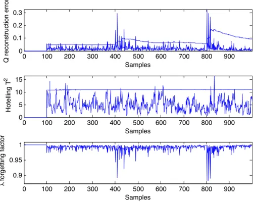
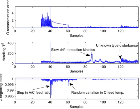
1.1 Knowledge Discovery in Databases - data driven development . . . 2 2.1 Process data in considered scenario of the AR process . . . 24 2.2 Hotelling T2, Q metrics and value of forgetting factor in the
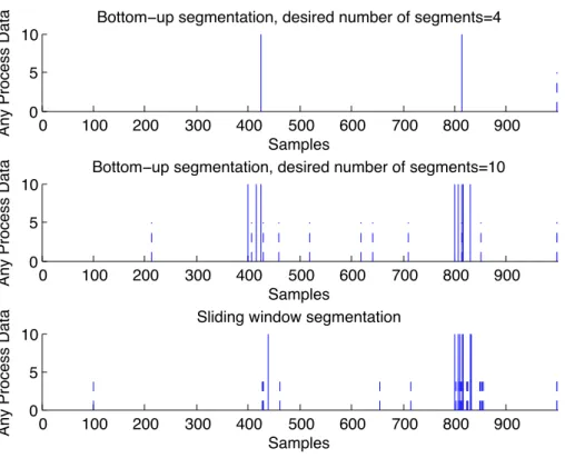
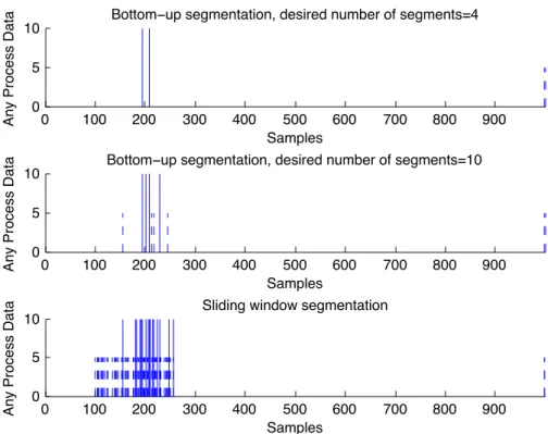
considered time scale of the AR process . . . 25 2.3 Results of different segmentation scenarios of AR process . . . 26 2.4 Q reconstruction error and Hotelling T2 metrics and value of
forgetting factor in the considered time scale using static PCA . . . 27 2.5 Results of different segmentation scenarios of AR process using
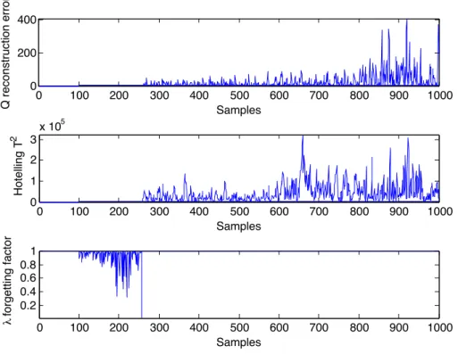
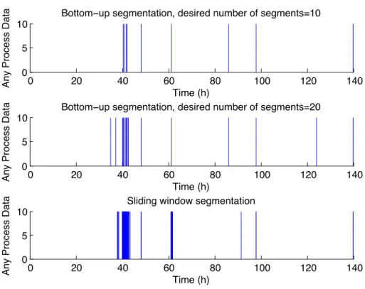
static PCA . . . 28 2.6 Hotelling T2, Q metrics and value of forgetting factor in the
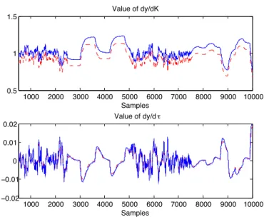
considered time scale of TE process . . . 30 2.7 Results of different segmentation scenarios of TE process . . . 31 3.1 Input-output process data of the first order process . . . 41 3.2 Sensitivities of the first order process. Comparison of thee
calculation methods. full line - analytical sensitivity using I.
approach, dotted line - analytical sensitivity using II. approach, dashed line - finite difference method . . . 43 3.3 Information content of binary signals with different periodic times . 44 3.4 Result of Fisher matrix based time-series segmentation and the
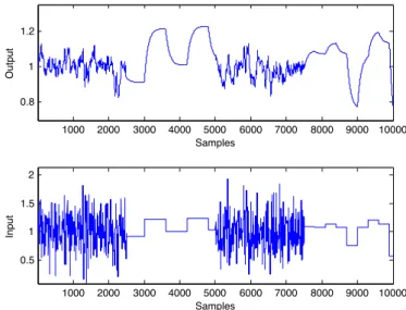
value of E criteria in the segments are also shown. . . 44 3.5 Process data used in the polymerization reactor example . . . 47 3.6 Result of segmentation for supporting to the identification of all
kinetic parameters . . . 48 3.7 Results of identification scenarios (full line - original data, dashed
line - the worst scenario, dashdot line - the best scenario) . . . 48
3.8 Result of segmentation for supporting the identification of exponential parameters . . . 49 3.9 Result of identification of the exponential parameters (full line -
original data, dotted line - best case, dashed line - worst case) . . . . 50 3.10 Result of segmentation for supporting the identification of
preexponential parameters . . . 51 3.11 Identification result focusing to preexponential parameters (full line
- original data, dotted line - best case, dashed line - worst case) . . . 51 4.1 Topology of the district heating network . . . 61 4.2 Cell model of the heat exchanger . . . 62 4.3 Cell model of the production unit . . . 63 4.4 The layers of an economic optimization of an operating technology. 64 4.5 The outputs of the "operating process" and process model to the
same input signal . . . 67 4.6 The scheme of the implemented non-linear model predictive controller 68 4.7 Comparison of the transitions in outputs with initial parameters
(dashed line) and with the experimentally determined parameters (dotted line) . . . 71 4.8 Comparison of the transitions in inputs with initial parameters
(dashed line) and with the experimentally determined parameters (dotted line) . . . 72
List of Tables
3.1 Result of identification scenarios of determining all kinetic parameters 52 3.2 Result of identification scenarios of determining exponential
parameters . . . 53 3.3 Result of identification scenarios of determining preexponential
parameters . . . 54 4.1 ISE and IAE metrics for the considered control scenario . . . 72 4.2 Total movement of manipulated variables (IDU) in the considered
control scenarios . . . 73 A.1 Process disturbances for the Tennessee Eastmen Process . . . 91 A.2 Process variables used for dynamic PCA . . . 92 A.3 Result of identification scenarios of determining all kinetic parameters 93 A.4 Result of identification scenarios of determining exponential
parameters . . . 94 A.5 Result of identification scenarios of determining preexponential
parameters . . . 95
Chapter 1
Introduction
The economic crisis started in 2007 had serious effect also on the chemical industry and it is going to have effect in the next couple of years. New strategic direction has been evolved with the combination of increasing operation efficiency and high return on investment, especially in short term. The importance of energy saving, cost reduction solutions are highly appreciated and directions of these particular research fields are highly supported. The Advanced Process Control (APC), process monitoring and fault detection solutions can contribute to reach the goal either explicitly by e.g. reducing the utility consumption or explicitly by detection the occurred faults and being able to prevent further damages.
Information is a highly powerful resource to reach the previously mentioned goals. Huge amount of process data is archived thank to the highly automated chemical processes. These data archives have huge potential to extract valuable information from them for different purposes. Data collection usually takes place early in an improvement project, and is often formalized through a data collection plan, which often contains the following activities.
• Pre-collection activity (agreement on goals, target data, definitions, methods).
• Collection of data sets.
• Present Findings - usually involves some form of sorting analysis and/or presentation [1] .
In development projects of operating processes, targeted data collection usually means additional experiments to carry out. In lot of cases there is no option to make the best of extracting information from data collected in normal operation.
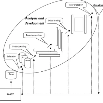
In Ref.[2] data collection methods and the use of historical process data in process improvement are very well described, having focus on Knowledge Discovery in Databases (KDD) framework. KDD has multiple steps to extract information from process data stored in databases, which are depicted in Figure 1.1.
!
"#$#%&'()!
*+#,+(%#--').!
/+0)-1(+20&'()!
30&0!2')').!
4)&#+,+#&0&'()! !"#$%&'(&)
*+,+)
) -./01)
)
/"+%2343)+"') '&5&%#67&",)
Figure 1.1: Knowledge Discovery in Databases - data driven development System identification, fault detection and process monitoring, time series analysis are considered as engineering tasks as part of KDD. The steps of this framework can be summarized as follows:
• Data selection: similarly to the precollection activity, the main application domain is developed and the main goal of KDD process is identified.
• Data pre-processing: the step of filtering and reconciliation of the collected data, in order to correct measurement errors e.g. due to measurement noise.
• Data transformation: the step of finding and performing features and application methods on process data for achieving the set of goals. This step prepares process data for the information extraction step.
• Data mining: extraction of information from the previously transformed process data. Various methods can be applied in this step, like clustering, regression, classification or time-series segmentation. The result might be
either expected and it confirms premisses or it can open brand new directions in process development.
Online detection of any misbehavior in the technology by analyzing the recently collected process data is a well defined engineering goal (it is called knowledge in KDD). PCA is well-known and applied approach in process monitoring.
Investigation of transient states needs dynamic PCA, since it can describe the dynamic behavior more accurately. Conventional PCA needs a huge amount of data for calculation of covariance matrix. Collecting enough process data to perform a new calculation of covariance matrix ruins the possibility of accurate online detection. Recursive PCA is for solving this problem since it needs only the latest process data and the latest covariance matrix to update covariance matrix. In this thesis, a combination and integration of the recursive and dynamic PCA is proposed and it is inserted into time series segmentation techniques. This results efficient multivariate time-series segmentation methods to detect locally linear homogenous operation ranges. E.g. this tool helps to reach the goal of online fault detection and separation of operation regimes, mentioned in the beginning of the paragraph. The similarity of time-series segments is evaluated based on the Krzanowski-similarity factor, which compares the hyperplanes determined by the PCA models.
Advanced chemical process engineering tools, like model predictive control or soft sensor solutions require proper process model. Parameter identification of these models needs historical data segregation of input-output data with high information content. This engineering goal is also a time-series segmentation task, like the detection of locally linear operation regimes in the previous case. Classical model based Optimal Experiment Design (OED) techniques can be applied to create experiments providing highly informative data. These solutions can also be utilized in the selection of informative segments from historical process data. In the thesis, a goal-oriented OED based (Fisher information matrix is the appropriate tool in OED) based time-series segmentation algorithm is introduced to fulfil this demand.
1.1 Time-series segmentation for process monitoring
Continuous chemical processes frequently undergo number of changes from one operating mode to another. The major aims of monitoring plant performance at process transitions are (i) the reduction of off-specification production, (ii) the identification of important process disturbances and (iii) the warning of process
malfunctions or plant faults. The first step in optimization of transitions is the intelligent analysis of archive (historical) and streaming (on-line) process data ([3]).
Fault and any misbehavior detection shall be performed by collecting and analyzing the input-output data together. This way, determination of events becomes possible where the correlation between the input and output process varies. Separation of input-output data during investigation of process events, and considering them as univariate time-series is impractical and misleads the engineer.
In this case we miss considering the process itself, which should be the object of the detailed investigation.
The detailed investigation of historical and streaming process data is recognized by the process monitoring and control industry and complex solutions have been provided for reaching these goals. Principal Component Analysis (PCA) and Partial Least-Squares (PLS) ([4]) and their different modifications have been applied more and more widespread ([5, 6, 7, 8]). Process monitoring approaches based on these methods conduct statistical hypothesis tests on mainly two indices, the Hotelling T2 and Q statistics in principal component and residual subspaces, respectively. Process failures, similarly to sensor faults ([9]) can be detected effectively by analyzing these metrics. Several approaches have been developed to extend the applicability of these methods for non-linear problems: by combining wavelet transformation and PCA tools ([10]) or by extension of PCA with kernel methods ([11]). Other multivariate process monitoring approach is the integration of qualitative trend analysis (QTA) and PCA ([12]). Correlation changes of process variables are detected by QTA, PCA assures to handle the multivariate characteristics of the process. In Ref. [13] a new methodology has been developed based on applying wavelets and combining it with Markov trees to enhance the process monitoring performance.
Nowadays nature inspired fault detection techniques become more and more widespread, like immune system or neural networks based methodologies ([14, 15, 16]). Artificial immune system based techniques mimic the operation of the human health defense system. "White blood cell" objects are defined and cloned to detect any faults in the operating technology ([15, 16]). It is similar to the principle of negative selection, where the immune system distinguish healthy body cells and foreign cells causing defections. The application of these methodologies starts with initialization where the definition of white blood cell objects is done. The next step is to choose a operation range or pattern for the learning algorithm, and to choose a test case to validate the result of the learning step. Highly experienced user has
the ability to select appropriate patterns and ranges for these purposes. Careful selection of these data sets is essential to avoid disadvantages of these methods like the constrained ability of recognition unlearnt scenarios. Artificial immune based techniques are applicable not just detecting but diagnosing the root causes of process faults. Artificial neural networks are also widely applied to establish even non-linear connection between input-output data, and to detect any misbehavior.
Recent techniques from this field are summarized in details in Ref [14].
Time-series segmentation methodologies are for segregating collected process data with considering pre-defined aspect. This method is often used to extract internally homogeneous segments from a given time series to locate stable periods of time, to identify change points ([17], [18]). Although in many real-life applications a lot of variables must be simultaneously tracked and monitored, most of the time series segmentation algorithms are based on only one variable ([3]).
One of the aims in this thesis is to introduce new time series segmentation algorithms that is able to handle multivariate data sets to detect changes in the correlation structure among process variables. PCA is the most frequently applied tool to discover information in correlation structure [19] like in field of fault detection [20]. As conventional PCA model defines a linear hyperplane and most production processes are non-linear, this approach is restrictively applicable for analyzing chemical technologies. To be able to locally linearize and this way follow the non-linearity of the process, we need to use the latest data of that operation regime to calculate proper models. This model calculation can be inaccurate if considering older data points which have no information content regarding to the recent PCA model. It might be necessary since computation of PCA models needs a numerous data points. The recursive computation way of PCA models ([21]) has the capability to use only the latest data points since the recent PCA model is yielded by updating the existing PCA model with the recent measurements. By applying the variable forgetting factor developed by Fortescue et al. [22], it is possible to determine the weight of the recently collected process data points in computation of the updated and proper PCA model. As conventional PCA is for analyzing static data, Ku et al. presented a methodology [23] called dynamic PCA (dPCA) to be able to handle the time dependency of the process data. In dynamic PCA the initial data matrix has been augmented with additional columns of process data collected in previous sample times. Combining the method of recursive PCA with dynamic PCA, a helpful tool is yielded to describe the dynamic behavior of multivariate dynamic systems throughout analysis of process data. Choi and Lee
developed an algorithm with kernel functions to capture the nonlinear behavior of chemical processes and combined it with dynamic PCA to describe the dynamical characteristics ([24]).
The developed segmentation algorithm can be considered as the multivariate extension of piecewise linear approximation (PLA) of univariate data sets ([25]).
Most of data mining algorithms utilize a simple distance measure to compare the segments of different time series. This distance measure is calculated based on the linear models used to describe the segments ([26]). The distance of PCA models could be determined using the PCA similarity factor developed by Krzanowski [27, 28]. By integrating the Krzanowski similarity measure into classical segmentation techniques new PCA based segmentation methods are resulted. As PCA has different metrics to describe the PCA model (Hotelling T2 statistics, Q reconstruction error) in the further research the possibilities of utilization of these metrics are going to be investigated in details.
In the previously mentioned nature inspired methodologies ([14, 15, 16]) need learning and validating process to become ready to be used to detect and recognize process misbehaves and faults. Unlike these tools, the developed dPCA based technique needs only initialization by defining the initial variance-covariance matrix. As the developed time-series segmentation based process monitoring approach is based on continues update of PCA models and detection of differences between the PCA models, learning and validating process can be skipped. The need of PCA model update means changes in the correlation structure of input-output variables. When fault diagnosis is needed beside the fault detection, supervised learning has to be applied to learn the different fault scenarios.
The application way of the developed algorithm is presented on a simple auto-regressive (AR) system and on the benchmark of Tennessee-Eastman (TE) problem. Multivariate statistical tools are mostly evaluated and tested on Tennessee- Eastman problem in chemical and process engineering practice. TE process is applied for various goals, like [29] developed and tested his branch and bound methodology for control structure screening. In field of process monitoring several intuitive methodologies are developed and presented throughout TE example, like Bin Shams et al. [30] introduced his method based on CUSUM based PCA. The Independent Component Analysis is also widely applied for monitoring process performance, like Lee et al. [31], who also generated test faults for his methodology using the TE process. The application of one of the most intuitive methodologies is also presented using this benchmark, where Srinivasan [32] developed a fault
detection framework based on dynamic locus analysis for online fault diagnosis and state identification during process transitions.
1.2 Time-series segmentation based on information content
Most of advanced chemical process monitoring, control, and optimization algorithms rely on a process model. Some parameters of these models are not knowna priori, so they must be estimated from process data either collected during targeted experiments or normal operation (historical process data). The accuracy of these parameters largely depends on the information content of data selected to parameter identification [33]. So there is a need for an algorithm that can support information content based selection of data sets. As we saw previously, targeted selection of suitable data sequences is a time-series segmentation task.
Shannon defined the information content first in the field of communication [34]. An essential problem of communication was to reproduce a message in the end point that was coded in the starting point. In Shannon’s theory, entropy measures the information content of the message. It simply measures the uncertainty in the message just like Gibbs entropy measures the disorder in a thermodynamic system.
Information content in mathematical model identification is a specific characteristic of the chosen process data set: measures the "useful" variation of the model input data set which causes significant changes in the model output data set.
"Useful" variation helps us the determine the model parameters using identification techniques. Obviously, the more "useful" variation we have, the higher information content the considered data set possesses.
Extraction of highly informative time-series segments from historical process data requires novel, goal-oriented time-series segmentation algorithm. One of the key ideas in this thesis is the propose the utilization of tools of optimal experiment design (OED) in this new field. Franceschini [35] provides an overview and critical analysis of this technique. Tools of optimal experiment design are applicable to measure the information content of datasets [36] regarding to a pre-defined process model. Usually OED is an iterative procedure that can maximize the information content of experimental data through optimization of (process model) input profiles [37]. OED is based on a sensitivity matrix - so-called Fisher information matrix, which is constituted from partial derivatives of model outputs respect to changes
of selected model parameters. Tools and methods of sensitivity analysis are summarized in details by Turanyi [38]. The information content of the selected input data sequence can be measured by utilizing A, E or D criteria [36, 39] based on the sensitivity based Fisher information matrix. As each criterion is an aggregate metric based on the Fisher information matrix, they all have their strengths and weaknesses. In order to mitigate these drawbacks and being able to combine the advantages of these metrics, Telen et al. [40] developed a multi-objective approach which enables to combine two optimization criteria. Experimental design procedures for model discrimination and for estimation of precise model parameters are usually treated as independent techniques. In order to match the objectives of both procedures, Alberton et al. [41] proposes use of experimental design criteria that are based on measures of the information gain yielded with new experiments.
Experimental design techniques are also available to design optimal discriminatory experiments [42], when several rival mathematical models are proposed for the same process. Performing additional experiment for each rival model may undermine the overall goal of optimal experimental design, which is to minimize the experimental effort. Brecht et al. deals with the design of a so-called compromise experiment [42], which is an experiment that is not optimal for each of the rival models, but sufficiently informative to improve the overall accuracy of the parameters of all rival models. Alberton et al. presents a new design criterion for discrimination of rival models [43], taking into account the number of models that are expected to be discriminated after execution of the experimental design.
In this thesis OED techniques are utilized to extract informative segments from a given time-series and separate different segments to identify different models or parameters. At first the input signal should be separated into sets of input sequences as the basis for constituting the Fisher information matrix. Fisher matrix can possess surplus information - not just the quantity of the information but its direction in the considered information space. Time series segments with similar information content can be described by similar information matrices. With the help of Krzanowski distance measure [27] it is possible to determine the similarity of Fisher matrices by direct comparison of them. In the thesis a novel and intuitive time-series segmentation algorithm is introduced for supporting to identify parameter sets from the most appropriate time frame of historical process data. This leads to reduction in the cost and time consumption of parameter estimation.
1.3 Economic based application of experiment design
The information extracted from plant historians is highly suitable for supporting controller design. Thanks to the general non-linear behavior of chemical processes of it is very difficult to find the right tuning parameters of the controllers in the whole operation range. In spite of the nonlinearity of processes most of the controllers are installed with linear algorithms. The right parameters for the production (e.g. set-points, tuning parameters of controllers, valve positions) are determined experimentally using the intuition of engineers. The response of the non-linear process is approximated with linear models and each linear model is valid only within a narrow operation range. A model library is needed to be created to characterize the operating process in the whole operation range [44].
The possibilities of the model library conducted to the demand of re-determining controller tuning parameters even if it is an iterative process like iterative learning control in batch processes [45, 46]. A know-how is necessary to fulfill these requirements, which is easy to implement even in case of operating model predictive controllers (MPCs). The tools of classical experiment design techniques can reach all these goals.
The production in the chemical industry represents a typical example of a multiproduct process. One reactor is used for producing various products and changes of production circumstances is handled by control algorithms. During transitions between products, off-specification products are produced. This product is generally worth less than the on-specification material (which fulfill all the commercial and quality requirements), therefore it is crucial to minimize its quantity. From control algorithm point of view, it means to find correct tuning parameters which enable reaching new setpoints. Beside the importance of the process transients, an on-specification product can be produced under varying circumstances and at varying operating points, which motivates us to find the (e.g.
economically) optimal operation point in production stages.
The demand for time and cost reduction of grade transitions inspire researchers to find more and more innovative solutions [47, 48]. Optimization of complex operating processes generally begins with a detailed investigation of the process and its control system [31]. It is important to know how information stored in databases can support the optimization of product transition strategies. How hidden knowledge can be extracted from stored time-series, which can assure additional possibilities to reduce the amount of off-grade products. The optimization of
transition is a typical task in process industry [49]. Modern control algorithms and strategies are available to handle these tasks effectively. The determination of the tuning parameters of these algorithms are quite difficult, time and cost consuming and experimental process.
One of the common experimentation approaches is One-Variable-At-a-Time (OVAT) methodology, where one of the variables is varied while others are fixed.
Such approach depends upon experience, guesswork and intuition for its success.
On the contrary, tools like design of experiments (DoE) permit the investigation of the process via simultaneous changing of factors’ levels using reduced number of experimental runs. Such approach plays an important role in designing and conducting experiments as well as analyzing and interpreting the data. These tools present a collection of mathematical and statistical methods that are applicable for modeling and optimization analysis in which a response or several responses of interest are influenced by various designed variables (factors) [50].
There are typical grade/ operation "sequences" during running the processes so it is possible to handle them like a "batch" in the pharmaceutical industry.
This approach allows us to integrate the iterative learning control scheme into the optimization of the grade transition. It means that the optimal grade change strategy - by manipulating the tuning parameters of the controller - could not be found in one step but iteratively. The experimental design techniques need low number of iteration during optimization, so they are beneficial if combined with the iterative learning control theory.
In this thesis the applicability of experimental design technique is going to be examined. This approach will be proven to be appropriate for finding the right tuning parameters of an MPC controller. The aim of the case study is the reduction the time consumption of transitions.
Chapter 2
On-line detection of homogeneous
operation ranges by dynamic principal component analysis based time-series segmentation
Any development in process technologies should be based on the analysis of process data. In the field of process monitoring the recursive Principal Component Analysis (PCA) is widely applied to detect any misbehavior of the technology. Recursive computation of PCA models means combining the existing PCA model with the recent process measurements and it results the recent PCA model. The investigation of transient states needs dynamic PCA to describe the dynamic behavior more accurately. By augmenting the original data matrix of PCA with input-output data from previous sample times conventional PCA becomes "dynamised" to catch the time-dependency of process data. The integration and combination of recursive and dynamic PCA into classic time series segmentation techniques results efficient multivariate segmentation methods to detect homogenous operation ranges based on either historical or streaming process data. By these new multivariate time- series segmentation techniques we can support process monitoring and control by separation of locally linear operation regimes. The performance of the proposed methodology is presented throughout an example of a linear process and the commonly applied Tennessee Eastman process.
2.1 dPCA based multivariate time series segmentation
In the process industry we need to be able to connect manufactured products and the operation regimes in which they were produced. It has several advantages: it becomes possible to detect occurrences of different disturbances, there is chance to find a suitable operation regime for model parameter estimation, etc. The first step on this way should be the analysis of historical process data. The correlation between input-output data is determined by the process itself, the output process data shall be handled as complex function of input process data. Hence input- output datasets can be considered as a multivariate time-series. Dynamic principal component analysis is a suitable for extending the classical univariate time-series approaches for multivariate cases and it can be the basis for developing a toolbox to fulfill demand of segregating the homogeneous operation regimes.
The chapter is organized as follows: in the rest of this section the main parts of the developed dynamic PCA based time-series segmentation methodology is going to be introduced. First, the principles of time series segmentation is explained in details. Then the connection of classical and dynamic principal component analysis and time-series segmentation is presented. In the end of the section integration of the most important components, like recursive computation of covariance matrices and Krzanowski similarity measure is shown and then the detailed summary of developed algorithm is introduced.
2.1.1 Multivariate time series segmentation algorithms
A multivariate time seriesT ={xk = [x1,k, x2,k, . . . , xn,k]T|1≤k ≤N}is a finite set of N n-dimensional samples labelled by time points t1, . . . , tN. A segment of T is a set of consecutive time points which contains data point between segment boarders of a and b. If a segment is denoted as S(a, b), it can be formalized as:
S(a, b) = {a ≤ k ≤ b}, and it contains data vectors of xa,xa+1, . . . ,xb. The c- segmentation of time series T is a partition of T to cnon - overlapping segments STc ={Si(ai, bi)|1≤i≤c}, such thata1 = 1, bc =N, andai =bi−1+ 1. In other words, anc-segmentation splitsT tocdisjoint time intervals by segment boundaries s1 < s2 < . . . < sc, whereSi(si, si+1−1).
The goal of the segmentation procedure is to find internally homogeneous segments from a given time series. Data points in an internally homogeneous
segment can be characterized by a specific relationship which is different from segment to segment (e.g. different linear equation fits for each segments).
To formalize this goal, a cost function cost(S(a, b)) is defined for describing the internal homogeneity of individual segments. Usually, this cost function cost(S(a, b))is defined based on distances between actual values of time-series and the values given by a simple function (constant or linear function, or a polynomial of a higher but limited degree) fitted to data of each segment (the model of the segment). For example in [51, 52] the sum of variances of variables in segment was defined ascost(S(a, b)):
cost(Si(ai, bi)) = 1 bi−ai+ 1
bi
X
k=ai
kxk−vi k2, (2.1)
vi = 1 bi−ai+ 1
bi
X
k=ai
xk,
wherevi the mean of the segment.
Segmentation algorithms simultaneously determine parameters of fitted models used to approximate behavior of the system in segments, and ai, bi borders of the segments by minimizing the sum of costs of the individual segments:
cost(STc) =
c
X
i=1
cost(Si(ai, bi)). (2.2) My aim in this thesis is to extend the univariate time series segmentation concept to be able to handle multivariate process data. In the simplest univariate time-series segmentation case the cost of Si segment is the sum of the Eucledian distances of the individual data points and the mean of the segment.
In the multivariate case a covariance matrix is calculated in every sample time, so the result is a "covariance matrix time-series". The cost of Si segment is the sum of the differences of the individual PCA models to the mean PCA model calculated from the mean covariance matrix. The similarities or differences among multivariate PCA models can be evaluated with the PCA similarity factor,SimP CA, developed by Krzanowski [27, 28]. It is used to compare multivariate time series segments. Similar to Eq(2.1), the similarity of covariance matrices in the segment to the mean covariance matrices can be expressed as the cost of the segment. Consider Si segment withai andbi borders. A covariance matrix (Fk) is calculated in every sample point between the segment boarders, ai ≤ k ≤ bi The mean covariance
matrix can be calculated as:
FT(ai, bi) = 1 bi−ai+ 1
bi
X
k=ai
Fk (2.3)
whereFkcovariance matrix is calculated in thekthtime step from the historical data set having n variables. PCA models of Si segment consist of p principal components each. The eigenvectors ofFT andFk are denoted byUT ,p and Uk,p, respectively. The Krzanowski similarity measure is used as cost of the segmentation and it is expressed as:
SimP CA(ai, bi) = 1 bi−ai+ 1
bi
X
k=ai
1
ptrace UTT ,pUk,pUTk,pUT ,p
(2.4) In the equation above (Eq(2.4)) Uk,p is calculated based on the decomposition of theFk covariance matrixFk = UkΛkUTk into aΛk matrix which includes the eigenvalues ofFk in its diagonal in decreasing order, and into a Uk matrix which includes the eigenvectors corresponding to the eigenvalues in its columns. With the use of the first few nonzero eigenvalues (p < n, where n is the total number of principal components, p is the number of applied principal components) and corresponding eigenvectors, PCA model projects correlated high-dimensional data onto a hyperplane of lower dimension and represents relationship in multivariate data.
Since Fk represents the covariance of the multivariate process data in the kth sample time, the calculation ofFkcan be realized in different ways, e.g. in a sliding window or recursive way. In this thesis Fk is calculated recursively on-line, the detailed computation method is presented in Section 2.1.3.
The cost function Eq(2.2) can be minimized using dynamic programming by varying the place of segment borders, ai and bi (e.g. [52]). Unfortunately, it is computationally too expensive for many real data sets. Hence, usually one of the following heuristic, most common approaches are followed [25]:
• Sliding window: A segment is continuously growing and the recently collected data point is merged until the calculated cost in the segment exceeds a pre-defined tolerance value. For example a linear model is fitted on the observed period and the modeling error is analyzed.
• Top-down method: The historical time series is recursively partitioned until some stopping criteria is met.
• Bottom-up method: Starting from the finest possible approximation of historical data, segments are merged until some stopping criteria is met.
In data mining, bottom-up algorithm has been used extensively to support a variety of time series data mining tasks [25] for off-line analysis of process data.
The algorithm begins with creating a fine approximation of the time series, and iteratively merge the lowest cost pair of segments until a stopping criteria is met.
When the pair of adjacent segments Si(ai, bi) and Si+1(ai+1, bi+1) are merged a new segment is considered Si(ai, bi+1). The segmentation process continues with calculation of the cost of merging the new segment and its right neighbor and its left neighbor (Si−1(ai−1, bi−1)segment) and then with further segment merging.
To develop a multivariate time-series segmentation algorithm which is able to handle streaming process data, sliding window approach should be followed. After initialization, the algorithm merges recently collected process data to the existing segments until the stopping criterion is met. The stopping criterion is usually a determined value of the maximal merging cost.
This algorithm is quite powerful since merging cost evaluations requires simple identifications of PCA models which is easy to implement and computationally cheap to calculate. The sliding window method is not able to divide up a sequence into a predefined a number of segments; on the other hand this is the fastest time- series segmentation method.
2.1.2 Application of PCA for analyzing dynamic systems
The classical PCA is mainly for exploring correlations in data sets without any time dependency. In some industrial segments (e.g. in some polymerization processes) time consumption of process transitions is in the same order of magnitude with the length of a steady state operation. Hence it is crucial to be able to analyze and extract information from data sets collected in transitions. The demand of being able to handle time dependency of the collected process data motivated Ku and his colleagues [23] to dynamize the static PCA for the needs of dynamic processes.
Consider the following process:
yk+1 =a1yk+. . .+anayk−na +b1uk+. . .+bnbuk−nb+c (2.5) where ai, bj (i = 1, . . . , na, j = 1, . . . , nb) and care vectors of constants, na andnb show the time dependency of process data,uk is the vector ofkthsample of
(multivariate) input andykis the output (product) vector in the same time. Ku et al.
[23] pointed out that performing PCA on theX = [y,u]data matrix preserves the auto and cross correlations caused by time variance of the time series such as the ones above.Thus, Ku et al. [23] suggested that theXdata matrix should be formed by considering the process dynamics at every sample point. Generally speaking, every sample point should be completed with the points they are depending on, i.e.
the past values:
X=
yk . . . yk−na uk . . . uk−nb
yk+1 . . . yk−na+1 uk+1 . . . uk−nb+1
... . .. ... ... . .. ... yk+m . . . yk−na+m uk+m . . . uk−nb+m
(2.6)
Process dynamics create relationship between inputs and outputs - relations are preserved under PCA - and a model can be fitted with a model certain order. Usually na +nb is higher than the model order that is fitted to the data set. na +nb is equal to the total number of principal components, n. Performing PCA on the modified data matrix moves unwanted correlations to noise subspace. Possible combinations of time dependence are presented in the data matrix and we select the most important combinations of these by using PCA. First zero (or close to zero) eigenvalue shows linear relationship between variables revealed by the eigenvector belongs to this eigenvalue. The method of dynamizing the PCA is recognized and effectively applied in the field of process model identification ([53, 54]) so it proves the relevance and applicability of dPCA in handling even streaming multivariate process data.
2.1.3 Recursive PCA with variable forgetting factor
To detect changes in the process dynamics in time, we have to reach the acceptable resolution which needs us to compute a PCA model in every sample time.
This is also necessary in sliding window segmentation technique or in the fine approximation of bottom-up approach. To reach this goal the method of recursive PCA is applied ([55, 21]). This is based on recursively updating the variance- covariance matrix (XTkXk), whereXkis a data matrix (like Eq (2.6)) in thekthtime step comprising pvariables andn samples, proposed by Li et al. [21]. Recursive calculation of the (d)PCA model help us to avoid the excessive expansion of data matrix caused by frequently collected process data. This is a well-known issue in
e.g. adaptive control [22].
The proposed algorithm for recursive computation of covariance matrices is as follows:
1. Initialization
Nominal data, X, is defined, as previously introduced. The data set is normalized to zero mean and unit standard deviation, X0. Vectors of mean values, x0, and standard deviation, s0, are saved. The initial variance- covariance matrix can be expressed as:
F0 = XT0X0
l−1 (2.7)
wherelis the number of initial samples.
The initial forgetting factor is defined as:
λ0 = 1−(1
l) (2.8)
2. Application of variable forgetting factor in calculation of new covariance matrices.
(a) The new vector of measurements,xk, is collected. The new mean vector is calculated as:
xk =λk−1xk−1+ (1−λk−1)xk (2.9) (b) The difference of the new mean,xk, and the old mean,xk−1, is stored in δxk. It is necessary since the recursive calculation of process variance (σ) is as follows:
σk =λk−1(σk−1+δx2k) + (1−λk−1)(xk−xk)2 (2.10) The standard deviation in sample timek can easily be calculated from the process variance.
(c) Next step is to normalize recently collected process data, xk, using previously calculated mean, xk, and standard deviation, sk. The recursive calculation of variance-covariance matrix is formulated as:
Fk=λk−1Fk−1+ (1−λk−1)(χTkχk) (2.11) whereχkis the normalized process data vector,χk = xks−xk
k .
(d) The final step in the recursive calculation loop is to calculate the value of the variable forgetting factor,λk. To calculate the value of the forgetting factor Fortescue [22] proposed an algorithm, it is calculated as follows:
λk = 1− [1− Tpk2]ep2k
√nk−1
(2.12) where p is the number of applied principal components, nk is the asymptotic memory length at(k−1), theT2is the HotellingT2metric at sample pointkand the error termekis theQmetric, the reconstruction error at sample pointkpresented in [55].
As the forgetting factor decreases, the recent observation get more weight in calculation of updated variance-covariance matrix with less weight being placed on older data. Hence it is one of the basic component for quick adaptation of dPCA models to describe the correlation structure in the changed operation regime. It can be handled as an indicator where dPCA model needs to be updated rapidly to describe the new relationship of process variables.
2.1.4 Recursive dPCA based time-series segmentation
The dynamic principle component analysis was introduced in the previous section as an approach to be able to handle the time dependence of the collected process data (Eq (2.6)). Applying the recursive calculation method (Eq (2.11)) a new dPCA model becomes accessible in each sample point. With the application of the variable forgetting factor (Eq (2.12)) it becomes possible to exclude as much information as included by the recent measurements.
The next step is to find a valid dPCA model for each segment - so-called mean model (Eq(2.3))- and compare the recently computed dPCA models to the mean model. The comparison of dPCA models represented by the variance- covariance matrices become possible by using the Krzanowski similarity measure (Eq (2.4)). Application of segmentation algorithms become available by the help of this similarity measure so thus the segments with different dynamic behavior can be
differentiated.
For off-line application the bottom-up segmentation method is applied. The pseudocode for algorithm is shown in Algorithm 2.1.
Algorithm 2.1Bottom-up segmentation algorithm
0: Calculate the covariance matrices recursively and split them into initial segments (define initialaiandbi segment boundary indices).
0: Calculate the mean model of in the initial segments (Eq(2.3)).
0: Calculate the cost of merging for each pair of segments:
mergecost(i) =Sim(ai, bi+1)
whileactual number of segments>desired number of segmentsdo Find the cheapest pair to merge:
i=argmini(mergecost(i))
Merge the two segments, update theai, biboundary indices Calculate the mean model of in the new segment (Eq(2.3)).
recalculate the merge costs.
mergecost(i) = SimP CA(ai, bi+1)
mergecost(i − 1) = SimP CA(ai−1, bi) where SimP CA is the Krzanowski distance measure
end while
The previously introduced bottom-up segmentation technique is applied as off- line time-series segmentation procedure. There are some difficulties during the application of this methodology like the determination of initial and desired number of segments. Stopping criterion of segmentation procedure can be either the desired number of segments (as introduced in Algorithm 2.1) or reaching the value of a pre defined maximal cost. If the number of the desired segments are lower than the number of different operation regimes in the considered time scale, the result of the segmentation procedure might be misleading, since two or more similar, adjacent operation regime segments can be merged. If the number of the desired segments is too high, there will be the possibility to create false segments. False segments are subsegments of a homogenous segment and are not going to be merged. The introduced dPCA based bottom-up segmentation algorithm can handle this problem, since it is convergent. It means to reduce the possibility of false segments by "collecting" borders of the false segments next to the border of the homogeneous operation regime. In details: Assume that a process transient causes changes in the correlation structure of input-output variables. So we are getting from one operation range to an other. When the process is adapting to new operation conditions the dPCA models are continuously updated. Thanks to the variable forgetting factor the speed of this adaptation is "fast". Similarities of continuously
computed dPCA models to the average dPCA model of a homogeneous segment are low during process adaptation. It is because, correlation of input and out variables is continuously changing in transient state until it gets to the new homogeneous operation range. Hence merge costs are the highest in the transient time stamps. As transient state typically cannot be described by a linear PCA model, every PCA model is significantly different from each other as well as different from PCA model in homogeneous operation. It is the cause of the convergence. Taking the value of forgetting factor into consideration in segmentation algorithms, remaining superfluous and misleading segment boarders can be distinguished. If the value of forgetting factor is rapidly decreasing and exceeds a certain limit, the boundary of the segment could be considered as a valid segment boarder, otherwise it might be considered as a false segment boarder. The number of initial segments is up to definition but it can be stated that finer approximation of the time series result more sophisticated result. Too fine approximation might ruin the robustness of the algorithm. The only constraint is the number of data points, which have the ability of defining the model of the initial segments. In this particular segmentation methodology it is possible to define one variance-covariance matrix as an initial segment.
For on-line application the sliding window segmentation method is suitable.
The pseudocode of developed algorithm for multivariate streaming data is shown in Algorithm 2.2.
Algorithm 2.2Sliding window segmentation algorithm
0: Initialize the first covariance matrix.
whilenot finished segmenting time seriesdo Collect the recent process data.
Calculate recent the covariance matrix recursively.
Determine the merge cost (SimP CA) using the Krzanowski measure.
ifS < maxerrorthen
Merge the collected data point to the segment.
Calculate the mean model of in the segment (Eq(2.3)).
else
Start a new segment.
end if end while
The possible differences in the results of the off-line and on-line algorithms is caused by the totally different operation methodology, since these approaches are heuristic in terms of minimizing the cost function in a segment. Thanks to the
heuristic approach certain parameters of the algorithms are needed to be defined (e.g. the number of segments in off-line case and the pre-defined error in case of on-line approach), which might also lead to different conclusions. In general, the results are quite similar, the possible differences make us investigate the roots of the small variance in them.
2.1.5 Application of confidence limits in dPCA based process monitoring
Confidence limits for Q reconstruction error and HotellingT2 statistics are usually defined in the commonly applied PCA based process monitoring techniques.
Augmenting the dPCA based time-series segmentation methodology with the utilization of the confidence limits lead to a complex process monitoring tool. It enables further and more investigation of the segmentation results. The confidence limits can be calculated recursively, similarly to the covariance matrix.
For HotellingT2statistics the confidence limit is defined as follows:
CLT2 = (r−1)2 r ·Bα,p
2,r−p−12 (2.13)
whereris the number of already collected and examined samples (r =k . . . m, see Eq (2.6 )),pis the number of principal components,αis the probability of false alarm for each point plotted on the control chartBα,p
2,r−p−12 is the(1−α)percentile of beta distribution with parametersu1 andu2 ([56, 57]).
For Q reconstruction error a similar limit can be defined with the following expression:
CLQ =θ1 ηα
pθ2h20
θ1 + 1 + θ2h0(h0−1) θ21
h1
0
(2.14) where
h0 = 1− 2θ1θ3
3θ22 (2.15)
and
θd=
n
X
i=p+1
γdi =trace(Rdk)−
pk
X
j=1
γjd (2.16)
whereηαis the normal deviation corresponding to the upper(1−α)percentile,
nis the number of variables,Rkis the covariance matrix in thekth sample time,γi is the eigenvalue of theithprincipal component.
As a covariance matrix is defined in every sample time, Hotelling T2 and Q prediction error could be applied as indicators of the process in every sample time.
Hotelling T2 represents the movement of the data in the multidimensional space, it contains important information about the process although the variables from which it is calculated is not independent. Utilizing the Krzanowski similarity factor to compare the defined hyperspaces, the homogeneous operation segments can be segregated.
2.2 Case studies
Each component of the proposed dPCA based time-series segmentation is investigated earlier, like the recursive computation of the covariance matrix ([21]) and variable forgetting factor, defined by [22]. The novelty in the proposed methodology is the new way of application and integration of the well-known methods.
The use of the proposed time series segmentation methodology will be demonstrated throughout a simple, multivariate process and as a second a much more complex and realistic Tennessee Eastman process. Data preprocessing methods are not used in these case studies as having synthetical data sets.
2.2.1 Multivariate AR process
Problem formulation
Consider the following process, as a benchmark of Ku et al. [23]:
zk = 0.118 −0.191
0.847 0.264
!
zk−1+ 1 2
3 −4
!
uk−1, (2.17)
yk =zk+vk (2.18)
whereuis the correlated input:
uk= 0.811 −0.226
0.477 0.415
!
uk−1+ 0.193 0.689
−0.320 −0.749
!
wk−1, (2.19)