P´ azm´ any P´ eter Catholic University
Doctoral Thesis
Kinematic measurement and analysis of human arm movements
Author:
Bence J´ozsef Borb´ely
Thesis Advisors:
Prof. Dr. P´eter Szolgay, D.Sc.
Dr. J´ozsef Laczk´o, Ph.D
A thesis submitted in partial fulfillment of the requirements for the degree of Doctor of Philosophy
in the
Roska Tam´as Doctoral School of Sciences and Technology Faculty of Information Technology and Bionics
Budapest, 2017
“Hope is not the conviction that something will turn out well but the certainty that some- thing makes sense, regardless of how it turns out.”
Vaclav Havel
Abstract
Quantitative measurement and analysis of human motion is a key concept in under- standing processes of our movement system. High precision measurement devices have advanced research activity in movement rehabilitation, performance analysis of athletes and the general understanding of the motor system during the last decades by making objective movement pattern comparison possible. This advancement was further accel- erated by model-based analysis approaches that enabled explicit characterization of the studied movement patterns.
From behavioral aspects, manual and visual target tracking represents an important part of human movements and show strong predictive behavior. Studies investigating predictive manual tracking so far focused on the explanation of finger acceleration as a function of the 2D-tracking error and on the relation between the 3D-tracking error and path curvature and spatial depth but did not consider the control of shoulder, elbow and wrist joints. In the first part of the thesis an experimental setup and procedure is presented to investigate how motor synergies (involving the aforementioned joints) differ between predictive and non-predictive movements. During the analysis, motor synergies are evaluated by applying the uncontrolled manifold method to the joint angle variance during 2D tracking of a target on a graphics tablet, where the 2D pen position is used as the hypothetical task variable by the method. It is investigated whether the synergy index – defined by variance ratios affecting and being irrelevant for the task variable – drops during predictive, internally driven tracking movements compared to visually, externally driven tracking movements.
In the second part of the thesis the development of a custom wearable measurement device for arm movements is presented. The prototype incorporates inertial sensors for movement recording to overcome issues accompanying measurements with line of sight methods and enables evaluation and analysis of various sensor calibration, filtering and sensor fusion algorithms in a fully customizable manner. In the last part, a novel kinematic algorithm is introduced that utilizes orientation information of arm segments (directly measurable with inertial sensors) to perform joint angle reconstruction in real- time.
Acknowledgements
First of all, I would like to thank my scientific advisorsP´eter Szolgay andJ´ozsef Laczk´o for their guidance, patience and valuable support during my studies.
I am very grateful to Tam´as Roska and Arp´´ ad Csurgay for the inspiring discussions and their unbroken enthusiasm and encouragement.
I acknowledge the collaboration withJ´ozsef Tak´acs,G´abor Fazekas andGy¨orgyi Stefanik during the first year of my studies.
I thank my former and current colleagues D´ora, Zsolt, Endre, Norbi, Zoli, J´anos, Csaba, Istv´an, Andr´as, Bal´azs, Antal, Vamsi, Dani, M´at´e, ´Ad´am, Zsolt, G´abor, Tam´as, Mikl´os, K´alm´an, Andr´as among others for the chats at lunch, their advices and for discussions about my ideas.
I would like to acknowledge the financial support from the P´azm´any P´eter Catholic University, Faculty of Information Technology and Bionics through the follow- ing grants: T ´AMOP-4.2.1.B-11/2/KMR-2011-0002, T ´AMOP-4.2.2/B-10/1-2010-0014, KAP-1.1-14/030 and KAP15-055-1.1-ITK.
I thank Katinka Tivadarn´e Vida for her always kind help and patience to make the administrative side of life easier, the work of the Dean’s Office, the Financial Department and the IT Department.
I spent over a year at the Research Training Group 1091 ”Orientation and motion in space” of the German Research Foundation (DFG) being part of the University Hospital of Ludwig-Maximilians-Universit¨at M¨unchen where I met a lot of great minds. I would like to thank Andreas Straube for his supervision and generosity and Thomas Eggert for his guidance and tireless help during my stay, I learned a lot from both of them.
Furthermore, I am grateful to Maj-Catherine Botheroyd for her help in administrative and personal manners and all of the former colleagues for making this period a great experience.
I am very grateful to my mother and father and to my whole family who always believed in me and supported me in all possible ways.
Finally, I am especially grateful to my wifeMargar´etafor all of her love, patience, support and encouragement that gave me the strength to go on even in the hardest periods of this journey.
iii
Contents
Abstract ii
Acknowledgements iii
Contents iv
List of Figures vii
List of Tables viii
Abbreviations ix
1 Introduction 1
1.1 Motivation and scope . . . 1
1.2 Thesis outline . . . 3
2 Synergistic Control in Manual Tracking 5 2.1 Background . . . 5
2.2 Methods . . . 8
2.2.1 Subjects . . . 8
2.2.2 Experimental setup. . . 8
2.2.3 Design and procedure . . . 10
2.2.4 Data analysis . . . 14
2.3 Results. . . 16
2.3.1 Training block . . . 16
2.3.2 Test blocks . . . 17
2.4 Discussion . . . 18
2.4.1 Predictive tracking . . . 19
2.4.2 Adjustments of the synergy index. . . 20
2.4.3 The coice of cost function to model changing prior knowledge about the trajectory . . . 22
2.4.4 Conclusion . . . 26
3 A Development Framework for Arm Movement Measurements 28 3.1 Background . . . 28
3.2 Measurement device . . . 30
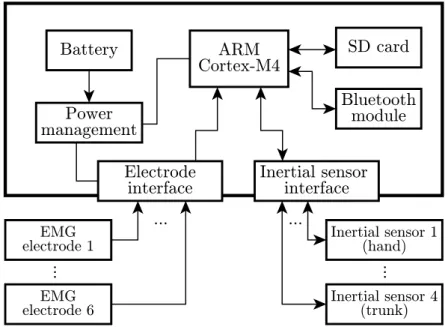
3.2.1 Base unit . . . 32
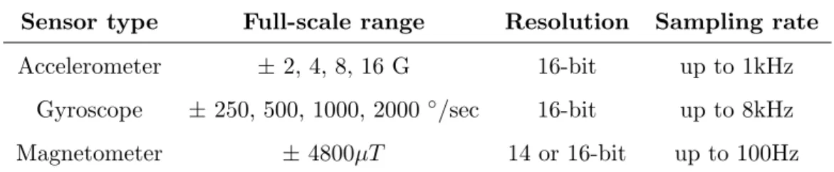
3.2.2 Inertial sensors . . . 33 iv
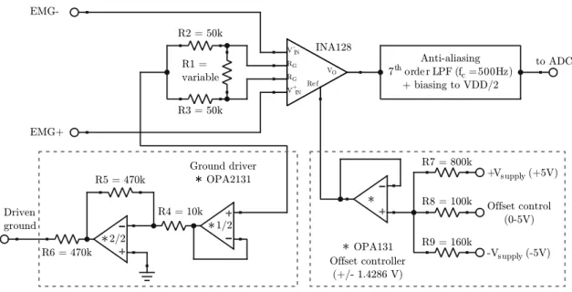
3.2.3 EMG frontend . . . 35
3.2.4 Hardware prototype . . . 38
3.3 Control software . . . 38
3.3.1 Data visualization . . . 40
3.3.2 Calibration of raw sensor measurements . . . 40
3.3.3 Calibration of sensor frame alignments . . . 46
3.3.4 Sensor fusion algorithm . . . 49
3.3.5 Anatomical joint angle reconstruction from sensor orientations . . 52
3.3.6 Standalone software version . . . 53
3.4 Conclusion . . . 53
4 Inverse Kinematics for Inertial Sensors 54 4.1 Background . . . 54
4.2 Methods . . . 56
4.2.1 Upper limb model . . . 56
4.2.2 Prototype markers . . . 61
4.2.3 Algorithm description . . . 63
4.2.4 Algorithm validation . . . 69
4.3 Results. . . 74
4.3.1 Accuracy . . . 74
4.3.2 Execution time . . . 75
4.4 Discussion . . . 77
4.5 Conclusion . . . 79
5 Conclusion 81 5.1 New scientific results . . . 81
5.2 Application of the results . . . 84
A Chapter 2: Mathematical Background 85 A.1 Partial compensation of planning noise . . . 85
A.2 Separation of feedforward and feedback components with complete knowl- edge of the target trajectory . . . 86
A.3 Extension to incomplete knowledge about the target trajectory . . . 87
A.4 Task error computed as weighted average of tracking errors in the target space and in the effector space . . . 89
A.5 Parameter settings for the simulation. . . 91
B Chapter 4: Mathematical Background 92 B.1 Definitions. . . 92
B.2 QR orthogonalization . . . 94
B.3 Auxiliary calculations for the shoulder . . . 95
B.4 MATLAB code for the compound rotation matrix of the shoulder . . . 96
B.5 Auxiliary calculations for the elbow. . . 97
B.6 MATLAB code for the compound rotation matrix of the elbow . . . 98
B.7 Auxiliary calculations for the wrist . . . 99
References 102 Journal publications of the Author . . . 102 Conference publications of the Author . . . 102 References cited in the thesis . . . 103
List of Figures
2.1 Experimental setup. . . 9
2.2 The presented target trajectories . . . 11
2.3 Measurement blocks of the experiment . . . 13
2.4 Time course of the tracking delay (A) and of the synergy index (B) in the training block . . . 17
2.5 Effects of the presentation mode on joint angle variances . . . 19
2.6 Simulation result of optimal feedback, applied to a simplistic tracking system with a 2D-effector space and a 1D-target trajectory . . . 23
3.1 Concept drawing of the measurement system . . . 31
3.2 Block diagram of the Base Unit . . . 33
3.3 Schematic drawing of the active EMG electrode frontend. . . 36
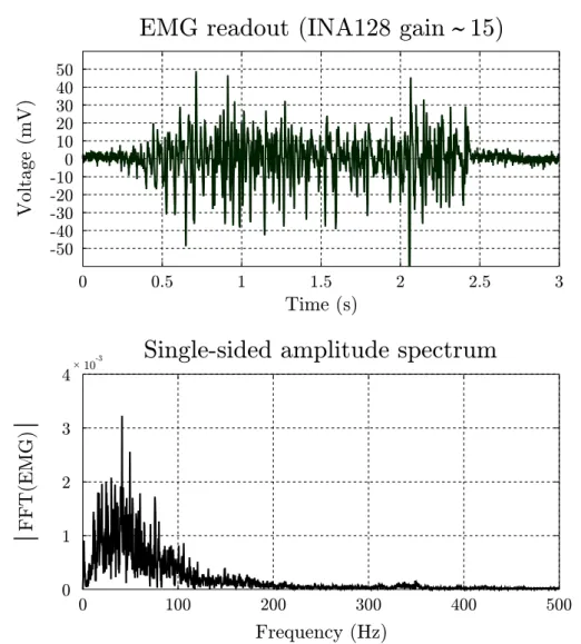
3.4 Test EMG measurement . . . 37
3.5 The prototype of the measurement device . . . 39
3.6 Single sensor data visualization . . . 41
3.7 Magnetometer calibration . . . 45
3.8 Experimental setup for sensor frame alignment calibration of inertial sensors 47 3.9 Example for manual movement segment selection . . . 47
3.10 Estimation of rotation axes based on accelerometer measurements . . . . 48
3.11 Sensor frame alignment results . . . 49
3.12 The effect ofβ on angle reconstruction . . . 50
4.1 Representations of the used upper limb model with reference poses and markers . . . 57
4.2 Visual representation of model-defined joint angle rotations (part 1) . . . 59
4.3 Visual representation of model-defined joint angle rotations (part 2) . . . 60
4.4 Representative screenshot of the tool developed for visual inspection of F(θflex, σ) (defined in Equation (4.6)) . . . 68
4.5 Representative simulated movement pattern used for algorithm validation 70 B.1 Visual representation of the definitions . . . 94
vii
List of Tables
3.1 Inertial sensor properties (MPU-9250) . . . 34
3.2 Zero motion offset values (MPU-9250) . . . 42
4.1 Memory footprint estimations (ARM builds) . . . 72
4.2 RMS errors . . . 76
4.3 Execution times. . . 77
B.1 Axis and angle notations. . . 92
viii
Abbreviations
fMRI functional MagneticResonanceImaging 2D 2-Dimensional
3D 3-Dimensional
UCM UnControlledManifold method DoF Degreesof Freedom
REX Real-timeEXperimentation system TRU 2Unpredictable 1TRajectory
TRn TRajectoryn, wheren∈ {1,2,3,4}
ANOVA ANanalysis Of VAriances HSD Honest Significant Difference LQG LinearQuadraticGaussian EMG ElectroMyoGram
MCU MicroControllerUnit CPU Central Processing Unit
SRAM StaticRandom AccessMemory MSPS MegaSamplesPerSecond ADC Analog toDigital Converter DAC Digital to Analog Converter I2C InterIntegratedCircuit SPI SerialPeripheralInterface
UART UniversalAsynchronous Transmitter / Receiver SDcard Secure Digital card
SDIO Secure Digital InputOutpout DMA DirectMemory Access BLE BluetoothLowEnergy
ix
RTOS Real-Time OperatingSystem FPU Floating PointUnit
MEMS Micro-Electro-MechanicalSystem IMU InertialMeasurementUnit
DMP Digital MotionProcessor FIFO FirstInFirstOut
DC DirectCurrent AAF Anti-AliasingFilter LPF LowPassFilter HPF HighPass Filter
FIR Finite ImpulseResponse
SAR SuccessiveApproximation Register DSP Digital SignalProcessing
SPP SerialPort Profile GUI Graphical User Interface DPS DegreesPerSecond PCB Printed CircuitBoard PC Personal Computer
PCA PrincipalComponentAnalysis LoS Lineof Sight
API ApplicationProgramming Interface IK InverseKinematics
XML EXtensibleMarkup Language PMx PrototypeMarker x
VMx VirtualMarker x
ANSI American National Standards Institute RMS RootMeanSquare
Chapter 1
Introduction
1.1 Motivation and scope
Movement is an essential part of our daily lives. It is so essential that we tend to forget its importance and take it for granted until we have to experience restrictions in our movement capabilities because of one of surprisingly many possible reasons. The human movement system is extremely complex from both anatomical and functional aspects, having centralized and distributed nature at the same time that assures adequate operation in very diverse situations.
As a simple example let us consider the case when someone touches a hot surface without any prior knowledge about its temperature: the movement starts with a voluntary part where motion planning, initiation and timing (among other functions) are performed in the interconnected neural structures of the cerebrum, cerebellum and brainstem, followed by the transmission of the execution commands to intermediate gateways in the spinal cord controlling the coordinated operation of different muscle groups through their α- motoneuron pools to make the arm extend and touch the surface. But simultaneously, the arm contains additional automatic built-in safety mechanisms (reflexes) that serve protecting purposes against various damaging factors – like burning the skin in our example – functioning independently of the central nervous system that results in far shorter reaction times than we could achieve voluntarily (generating an evasive movement even before we start noticing the pain). These reflexes are independent of cognitive processes as their functions are realized by direct wiring of neural pathways between the
1
sensor elements (muscle spindles, Golgi-tendons and various receptors of the skin) and theα-motoneuron pools in the spinal cord responsible for direct muscle control. Without going into further details (a comprehensive material on the topic can be found in [1]), even this simple example shows that the complexity and systematic structure of our movement system is an exciting, yet to be fully explored field of science.
Human movement science and selected fields of biomedical engineering aim to develop methodologies for proper examination of various aspects of our movement system. By elaborating quantitative measurement and analysis techniques of human movements, advancements in these fields have contributed to movement rehabilitation techniques [2], performance analysis of athletes [3] and general understanding of the motor system [4]
during the last decades by making objective movement pattern comparison possible. This advancement was further accelerated by model-based analysis approaches that enabled explicit characterization of the studied movement patterns [5].
It should be noted however that the possibilities for quantitative examination of the move- ment system in its whole are always constrained by the technology available to date. This is particularly true in the case of analysis of complex scenarios involving higher functional levels of the movement system (possibly including cognitive processes) that cannot be measured and tracked directly today. On the other hand, direct measurement of move- ment kinematics has became a standard process that can be performed with various movement analyzer systems using electromagnetic1, mechanical2, ultrasound3, optical4 or inertial5 technology. These measurements combined with additional recorded modal- ities (e.g. biopotential, force or (in rare cases) fMRI data) form the observation space in the wast majority of human movement analysis studies. As a consequence, conclusions about the underlying processes often have to be drawn incorporating simplified math- ematical models or previous behavioral observations into these studies, in addition to appropriate experimental design that excludes as many uncontrolled factors as possible.
As a subfield of movement science, understanding the nature and internal workings of human arm movements is of particularly high interest because we use our arms and hands in every situation when object manipulation is needed at any complexity level.
1Polhemus’ product portfolio – http://polhemus.com/motion-tracking/overview/
2Gypsy 7 – http://metamotion.com/gypsy/gypsy-motion-capture-system.htm
3Zebris’ CMS systems – http://www.zebris.de
4Vicon – https://www.vicon.com/; OptiTrack – http://www.optitrack.com/
5Xsens – https://www.xsens.com/
As a consequence, analysis of the underlying control methods in specific movement tasks and environmental conditions is a key aspect to gain more detailed knowledge of neural processes of our manual interaction with the environment.
In this thesis, three main topics are presented as an effort to contribute to the field of human movement science. The first topic covers an experimental study investigat- ing details of target tracking arm movements while the other two introduce engineering contributions to the field of measurement techniques by presenting the design and imple- mentation of a wearable measurement system along with an algorithm that establishes the connection between inertial measurements and model based analysis of movement kinematics.
1.2 Thesis outline
Chapter 2 introduces an experimental setup and procedure that was designed to in- vestigate how motor synergies differ between predictive and non-predictive movements.
Motor synergies were evaluated by applying the UCM method to the joint angle variance during 2D tracking of a target on a graphics tablet, where the 2D pen position was used as the hypothetical task variable. It was investigated whether the synergy index drops during predictive, internally driven tracking movements compared to visually, externally driven tracking movements. To address this question, tracking movements between pe- riodic (and pre-trained) and non-periodic presentation modes were compared, which are known to challenge predictive and visually driven tracking modes respectively.
Chapter 3 describes the engineering prototype development of a custom wearable mea- surement device based on my experiences with a movement analyzer system using ultra- sound technology. The prototype incorporates inertial sensors for movement recording to overcome issues accompanying measurements with the previous system (i.e. bulky setup, highly constrained measurement volume and low sampling rate) and enables evaluation and analysis of various sensor calibration, filtering and sensor fusion algorithms in a fully customizable manner.
An additional goal of this thesis is to extend the measurement and analysis workflow of human arm movements with a method that allows accurate and real-time calculation of anatomical joint angles for a widely used SIMM/OpenSim upper limb model when
measurements are performed with the developed prototype. For this purpose a custom kinematic algorithm is introduced in Chapter 4 that utilizes orientation information of arm segments (directly measurable with inertial sensors) to perform joint angle recon- struction in real-time.
Chapter 5 summarizes the results and concludes the thesis.
Chapter 2
Synergistic Control in Manual Tracking
The current chapter is based on the author’s articlce entitled “Motor synergies during manual tracking differ between familiar and unfamiliar trajectories”. [J1]
2.1 Background
Manual and visual target tracking represents an important part of human movements and shows strong predictive behavior. This becomes most obvious when comparing tracking onset delay with phase delays during pursuit of periodic movements [6] or when the movement continues after disappearance of the target [7]. Oculomotor and manual tracking responses affect each other [8,9] and seem to share predictive mechanisms [10].
Previous studies investigating predictive manual tracking focused on the explanation of finger acceleration as a function of the 2D-tracking error [11] and on the relation between the 3D-tracking error and path curvature and spatial depth [12] but did not consider the control of shoulder, elbow and wrist joints.
The Uncontrolled Manifold Method
The analysis of joint angle variability, especially its structural decomposition into task- relevant and task-irrelevant components with respect to hypothesized task variables, is
5
used to address redundancy in movement control mechanisms and was proposed by Scholz and Sch¨oner [13] as the ”Uncontrolled Manifold Method” (U CM). In this context the term ”task variable” does not imply that it was explicitly addressed in the instructions to the subject, but that the covariation in the effector space is optimized to stabilize this variable. The main concept of theU CM is to divide the total variance of the joint angles into two orthogonal sub-components that do and do not affect the proposed task variable.
The variance in the component which does not influence the task variable is called the
”uncontrolled variance” (VUCM) and can be used as an indicator of flexibility of the control system, while variance in its orthogonal component is called the ”controlled” or
”orthogonal variance” (VORT). The relative size of VUCM with respect toVORT, quantified by the so-called synergy index, can be used to characterize the stability of the task variable [14].
In more detail, after selecting a hypothetical task variable (e.g. the endpoint of the arm), the Jacobian matrix (J) can be obtained by the linearization of the task variable components expressed as a function of joint angles at the mean arm configuration. J expresses the linear mapping of differential changes in the 7-dimensional joint-space (∆ϕ) to differential changes of the task variable (∆ν) as shown in (2.1).
∆ν =J∆ϕ (2.1)
The basis of the uncontrolled manifold is named BUCM, that of the orthogonal subspace is calledBORT. BORT andBUCMcan be obtained from theQmatrix produced by the QR- decomposition of the transposed Jacobian matrix: [Q,R] = qr JT
;Q= [BORT,BUCM], where Qis orthogonal, BORT contains the first three and BUCM the last four columns of Q. The normalized variances of the projections on the two subspaces can be computed as shown in (2.2) and (2.3), whereDoFORT and DoFUCM denote the dimensions ofBORT
and BUCM, respectively. The synergy index is defined assi = VUCM
VORT
.
VORT = trace BTORTΣ BORT
DoFORT
(2.2)
VUCM= trace BTUCMΣ BUCM
DoFUCM
(2.3)
The normalization of the variances in the two subspaces to their respective dimensions is needed to ensure that, for a spherical distribution of the effector variables, the synergy index has the expected value of one, independent of the dimension of the task variable.
A large synergy index of the joint angle variance with respect to the task variable indicates that the ”bad” variance (affecting the task variable) is relatively small compared to
”good” variance (not affecting the task variable). It is important to note that this synergy index is specific for the chosen task variable and is not a general measure of covariation. The U CM method has been used to show the synergistic properties of the motor control system involving reaching [15, J3], finger coordination [16, 17, 18] and bimanual pointing tasks [19,20].
Optimal feedback control theory
According to the theory of optimal feedback control [21], motor synergies can be explained by a feedback controller minimizing costs expressed as the sum of two terms, a so called task-error depending on system states (joint angles and velocities), and a penalty on the control signals. This theory predicts that the synergy index decreases under open loop conditions, increases with increasing motor noise, and decreases with increasing sensory noise. Therefore, it can be expected that predictive and non-predictive movements which differ in precision (noise) and in the contribution of feedforward commands, show different motor synergies. However, such expectations of the theory are based on the assumption that the feedback controller is optimally adjusted to the actual conditions.
This chapter investigates how motor synergies differ between predictive and non- predictive movements. Motor synergies were evaluated by applying theU CM method to the joint angle variance during 2D tracking of a target on a graphics tablet, where the 2D pen position was used as the hypothetical task variable. It was investigated whether the synergy index drops during predictive, internally driven tracking movements compared to visually, externally driven tracking movements. To address this question, the presented work compares tracking movements between periodic (and pre-trained) and non-periodic presentation modes, which are known to challenge predictive or visually driven tracking modes respectively.
2.2 Methods
2.2.1 Subjects
Seven healthy subjects participated in the study (6 males, 1 female, age: 33.4 ± 12.4 years, mean ± standard deviation). All subjects had normal or corrected-to-normal vision. Five subjects had right hand dominance and 2 subjects had left hand domi- nance according to their preferential hand use during writing. All subjects performed the movements with their dominant hand. Because of marker measurement errors that could not be corrected, data from one of the right-handed male subjects were excluded from kinematic analysis of joint angle variances, but not from tracking performance anal- ysis. Subjects had given informed consent prior to participation in the experiment. The experimental procedure was in accordance with the Declaration of Helsinki and approved by the local Ethics Committee.
2.2.2 Experimental setup
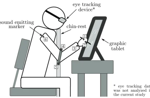
The subjects sat in front of a table which was mounted with a graphic tablet that featured an integrated display (Figure2.1, WACOM Cintiq 21UX, 43.2×32.4 cm, frame rate: 60 Hz) used for presentation of the target. The target was a white colored disk (diameter 1 cm) and moved in front of a gray background. The luminous sterance of the background luminance was about 20 cd/m2 and the target had a luminance of about 130 cd/m2. The sitting position of each subject was adjusted in the following way: (1) the body midline of the subject was aligned with the vertical midline of the graphic tablet, (2) the distance between the table on which the tablet was mounted and the subject’s chair, and the height of the chair were aligned to get the subject facing the graphic tablet’s midpoint orthogonally, (3) all possible target positions were within the anatomical range of motion of the subject’s measured arm, but not at extreme positions, and (4) to prevent trunk movements and to fixate the head, a supporting chin-rest with adjustable height was used. Post-hoc analysis revealed that the average movement amplitude of the acromion, defined as the largest distance between any pair of time samples of its 3D trajectory, was 1.48 ±0.25 cm (N=6). The viewing distance of the display was 40 cm.
sound emitting marker
6 1
3 2
4 graphic
tablet chin-rest
5
eye tracking device*
* eye tracking data was not analyzed in the current study
Figure 2.1: Experimental setup. Numbers 1-6 indicate ultrasound markers of the motion analysis system. The elbow bracelet that held the fourth and fifth markers was not attached to the chin-rest (as the figure may give an incorrect intuition), just to the subject’s arm. Subjects sat on a chair that was adjusted to provide stable fixation for their trunk. The target is depicted on the graphic tablet’s screen as a white disk.
The dashed line was never presented on the screen, it is only used in the figure to imply target movement. The eye tracking device is depicted in the figure because the measurement was part of an extended study that involved the analysis of eye movement data in addition to movement kinematics, however this modality was not included in
the analysis presented in the thesis.
Subjects were asked to track the target as accurately as possible with the pen of the graphic tablet using their dominant hand. Tracking performance was analyzed based on the pen data, recorded as 2D coordinates in the tablet’s reference frame. Arm movements were recorded by an ultrasound-based movement analyzer system (Zebris Medical, Isny, Germany) running at 33 Hz. The markers were attached to the following positions: (1) the metacarpophalangeal joint of the index finger, (2) the metacarpophalangeal joint of the little finger, (3) the center of the wrist. Markers (4) and (5) were attached to a bracelet directly above the elbow at the medial and lateral ends of the bracelet. Marker (6) was attached to the acromion. From these marker positions, a geometrical model of the arm with 7 degrees of freedom (DoF) was reconstructed in the tablet’s reference frame using a method described previously [J3]. The origin of this reference frame was the center of the tablet’s screen, its x and y axes coincided with the screen’s horizontal and vertical axes, while thez-axis was perpendicular to the screen pointing towards the subject (forming a right-hand coordinate system).
All data (target position, pen position and marker positions) were recorded by a com- puter running the real-time REX system [22], a QNX Neutrino RTOS-based software environment that is widely used to control neuroscience experiments1 and mapped at the common sampling rate of 1 kHz.
2.2.3 Design and procedure
As described in the introduction, the aim of the study was to investigate the effects of predictive and non-predictive tracking modes on movement performance and control. To achieve this, various 2D target trajectories were generated with a pseudo-random shape.
One of these trajectories (TR1) was only presented in periodic repetitions, whereas the other trajectories (TR2, TR3, TR4) were presented in a random order without repeti- tions. Moreover, in order to further stimulate predictive tracking of TR1, subjects were familiarized with this trajectory during an initial training block (seeMeasurement blocks for further details of the experimental design).
Trajectories
The 2D-velocities of the generated trajectories were based on sums of 5 harmonics with random phase and a base frequency corresponding to a period of 4 s. The 5 harmonics had frequencies of 0.25, 1, 1.75, 2.5, and 3.25 Hz. The peak velocities of the compo- nents were proportional to a Gaussian envelope with a value 1 at 0 Hz and decayed for higher frequencies. The decay of 3 dB was reached at 0.75 Hz. The frequency and magnitude values of the summed components were selected after visual inspection of various parameter combinations. Bothx and y velocities were generated independently.
Integrating these velocities yielded the 2D trajectories. These trajectories were then re- sampled nonlinearly to adjust the sampling distance (sd) according to (2.4), where V denotes the tangential velocity, r is the radius of curvature, and K and α are two free parameters [23]. This method is known as the two-thirds power law that describes an empirical relationship between the shape and the kinematics of free-hand and manual tracking movements [24,25], and it was applied here to assure that the subjects perceive the generated trajectories as natural as possible to avoid trajectory-induced error factors during the analyzed tracking movements.
1http://www.qnx.com/products/neutrino-rtos/neutrino-rtos.html?lang=en
sd
∆t =V =K r
1 +α·r 13
(2.4)
The variable ∆t specifies the sampling interval for the generated movement trace. The parameters K andαwere adjusted to achieve a mean tangential velocity of 10 cm/s and a ratio between the maximum and minimum tangential velocity of 2.
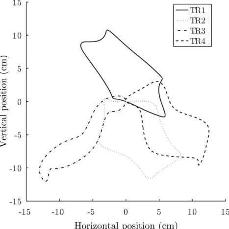
In this way 14 different random trajectories were generated independently from each other. Figure 2.2shows the 4 trajectories (TR1 to TR4) used for repeated presentation, as described in the next section. The remaining 10 trajectories (uniformly denoted as TRU) were used to introduce ”unpredictable” sections, as described below.
-15 -10 -5 0 5 10 15
-15 -10 -5 0 5 10 15
TR1 TR2 TR3 TR4
Vertical position (cm)
Horizontal position (cm)
Figure 2.2: The presented target trajectories. Closed traces were generated by integrating sums of 5 harmonics with a random phase and a base frequency correspond- ing to a period of 4 s. Labels (TR1-TR4) were assigned randomly to the generated
trajectories.
Measurement blocks
The smallest unit of the design was one presentation of a generated trajectory, which is referred to as a ”trial”. Trials were grouped into so-called ”sub-blocks”, followed by a pause of 4 s. The initial trials of these sub-blocks were not included in the analysis because they differed from the other continuation trials in the movement initiation required after the 4 s pause (see alsoData exclusion). The main experiment was composed of 6 blocks, each consisting of several sub-blocks as described below (for a graphical representation, see Figure 2.3). Blocks were separated by a break of about 5 minutes.
(1) In the first block, only the trajectory TR1 was presented in the so-called periodic training presentation mode as follows. The block consisted of 10 sub-blocks each con- taining 4 trials with periodic presentation of TR1. The purpose of this block was to make the subject familiar with the selected trajectory without introducing unwanted fatigue effects (pauses between sub-block executions). From the 40 presented trials, 30 continuation trials were analyzed.
(2) The periodic training block was followed by 5 test blocks, each presenting 12 sub- blocks. Six of these sub-blocks showed the non-periodic test presentation mode and contained the three trajectories TR2, TR3 and TR4 in a random order led by one of the unpredictable sections (TRU). Each of these 6 sub-blocks contained one of 6 possible permutations of TR2, TR3 and TR4. Alternating with the non-periodic test sub-blocks, 6 sub-blocks were inserted with TR1 in the so-called periodic test presentation mode.
This presentation mode was – apart from the vicinity to thenon-periodic test sub-blocks – identical to the periodic training mode. After exclusion of the initial trials of the periodic test sub-blocks and the initial, unpredictable sections of the non-periodic test sub-blocks, the five test blocks provided in total 90 trials (5 blocks ×6 sub-blocks ×3 trials) of periodic test trials (TR1), and 90 trials (5 blocks× 6 sub-blocks×3 trials) of non-periodic test trials (TR2, TR3 and TR4).
The specific structure of the non-periodic sub-blocks kept the subjects under the illusion of path randomness despite repetitive presentations of TR2-TR4. These repetitions were necessary to calculate joint angle variance-covariance which is the basis for the Uncontrolled Manifold Method.
TRAINING pause (4 s) pause (4 s)
...
pause (4 s)
TR1TR1TR1TR11 TR1TR1TR1TR12 TR1TR1TR1TR110
pause (4 s)
TRUTR3TR4TR21 pause (4 s)
TR1TR1TR1TR12 TRUTR3TR4TR23 pause (4 s) TR1TR1TR1TR14
...
pause (4 s) pause (4 s) TRUTR3TR4TR211 pause (4 s) TR1TR1TR1TR112
TEST (x5) Measurement block Periodic training / test sub-block Non-periodic test sub-block Non-periodic control sub-block
CONTROL pause (4 s) pause (4 s)
...
pause (4 s)
1TR1TR3TR4TR2TRU 2TRUTR4TR1TR2TR3 10TRUTR1TR3TR4TR2 Figure2.3:Measurementblocksoftheexperiment.Thesmallestunitofthedesignwasonepresentationofageneratedtrajectory,which isreferredtoasa”trial”.Trialsweregroupedintoso-called”sub-blocks”,followedbyapauseof4s.Themainexperimentwascomposedof6 blocks(TRAINING+5xTEST),eachconsistingofseveralsub-blocksofselectedtrajectories.ThemeasurementwiththeCONTROLblockwas performedafterthemainexperimenttotestwhetherdifferencesbetweenperiodicandnon-periodicpresentationswererelatedtothepresentation modesandnottodifferencesbetweenthetrajectories.ThebordersofthegraphicalboxesdenotingTR1-TR4refertothecorrespondingtrajectories showninFigure2.2
To test whether effects of periodic or non-periodic presentations were related to differ- ences between the trajectories rather than to the presentation modes a control experiment was performed on a different day, at least five weeks after the main experiment. This control consisted of a single ”non-periodic” block with 10 sub-blocks, each starting with one of the ”unpredictable” sections (TRU) followed by TR1, TR2, TR3 and TR4 in a random order. Thus, each trajectory was presented 10 times.
2.2.4 Data analysis
All data analysis was performed using MATLAB 7.9.0 (Mathworks, Natick, USA).
Tracking delay
Reduced tracking delay is the primary indicator for predictive versus visually driven tracking modes. Therefore, tracking delay was assessed by the time lag (ms) of pen position, evaluated by an algorithm used in previous studies [12]. In this algorithm, the hand-target distance was computed between the current hand position and the target position at any sampling point between 500 ms before and 100 ms after the current time.
The lag was defined as the time point at which the hand-target distance was minimal.
The average tracking delay was computed separately for eachsubject,block,presentation mode, and was averaged across all respective sampling points.
Data exclusion
The initial trial of each sub-block showed a tracking delay which started at a large value and rapidly decreased during the first half-cycle (2 s), due to movement initialization.
For example, in the initial trial of the first sub-block of the training the tracking delay decreased during the first 2 s from 292 ± 67 ms to 120 ± 53 ms. For that reason, all initial trials of all sub-blocks were excluded from the analysis. As a further step of preprocessing, the time courses of the tracking delays were checked for the occurrence of discontinuities (related to discontinuous mapping between hand position and target position). Since these discontinuities occurred only near to the start and the end of the trials, all data from a time window of 1 s around the trial start were excluded from the analysis.
Application of the uncontrolled manifold method
Like the average tracking delay, the uncontrolled manifold method was applied separately for each combination of the factorssubject,block, andpresentation mode, averaged across all respective sampling points. Following the method described in Section2.1, the synergy index was calculated with the pen position as the hypothetical task variable. Because of this, the arm configuration was constrained to 6 DoF since the z-component of the pen was constrained to the surface of the screen. Thus, the normalization factors were DoFORT = 2 and DoFUCM = 4. The total variance (Vtotal) of the joint angles was computed as the trace of the variance-covariance matrix (Vtotal = trace(Σ)).
Statistical analysis
To test whether tracking performance differed between the trajectories (TR1 - TR4), each of the dependent variables tracking delay, thetotal variance and thesynergy index of the control experiment was submitted to a repeated measures ANOVA with the factor trajectory (4 levels). For the main experiment each of these dependent variables was submitted to two repeated measures ANOVAs, one for the periodic training block and one for the test blocks. To analyze potential learning effects during the training con- secutive pairs of the 10 sub-blocks were pooled to form a repeated factor block number with 5 levels. To analyze the differences between periodic and non-periodic presentation modes and potential training effects in the test blocks, the two repeated measures fac- tors presentation mode (2 levels) and block number (5 levels) were used. Post-hoc tests were performed using Tukey’s HSD test. Effects were considered significant forα-errors p <0.05. α-errors different from this value are reported in the results to give a better intuition about the particular effect (e.g. p = 0.06 is a non-significant but marginal effect). Normality of the analyzed variables was checked with the Lilliefors test. Data sphericity was tested using Mauchly’s sphericity test. Wilks’ lambda multivariate test was applied if sphericity was not fulfilled. Descriptives of normally distributed variables are given as mean ± standard deviation and as median [interquartile range] otherwise.
Statistical results are reported in the following standard forms:
One-sided and paired T-test: T(df ) = T-value, p < p-value
Repeated measures ANOVA: F(dflevels, dferror) = F-value, p {<, =, >} p-value
where df means degrees of freedom and T-value and F-value are the values of the corre- sponding T and F statistics (for short descriptions of the methods and reporting stan- dards, please follow the links in the footnotes 2 3).
2.3 Results
Subjects reported that they felt familiar with the trajectory TR1 after the pure periodic training block of the main experiment, and that they also recognized it easily in the periodic test sub-blocks. In contrast, none of the subjects noticed that the trajectories TR2-TR4 were repeatedly presented. In the control experiment the tracking delay was 160 ± 20 ms, averaged across the 7 subjects, and showed a marginal effect of the fac- tor trajectory (main effect F(3,18) = 2.94; p = 0.06). However, none of the post-hoc tests reached significance (Tukey: p > 0.1), indicating that the different shapes of the trajectories did not have a major effect on tracking mode. This was further supported by the observation that neither the total variance (48.8 ±21.6 deg2) of the joint angles nor the synergy index (17.0±11.5) differed between the four trajectories (main effect of trajectory (F(3,15)< 0.43; p>0.73).
2.3.1 Training block
In the training block the tracking delay decreased from 116±41 ms during the first block to 94 ±33 ms in the last block (Figure2.4). This decrease was significant, as confirmed by the main effect of the factor block (F(4,24) = 3.68; p < 0.02). In the post-hoc test the tracking delay turned out to be longer in the first blocks than in the last three blocks (Tukey: p <0.05).
The overall mean of the synergy index during the training was 3.8 ± 2.0, significantly larger than 1 (one sided T-test: T(5) = 3.4; p <0.01), indicating that most of the joint angle variance was irrelevant for the pen position. There was also a significant main effect of the factor block number on the synergy index (F(4,2) = 50.9; p < 0.02). The third block showed a larger synergy index (5.77±4.71) than the last block (1.93±0.98;
2https://statistics.laerd.com/statistical-guides/dependent-t-test-statistical-guide.php
3https://statistics.laerd.com/statistical-guides/repeated-measures-anova-statistical-guide.php
1 2 3 4 5 60
100 140
Tracking delay(ms)
1 2 3 4 5
0 4 8 12
Synergy index
Block #
A
B
Figure 2.4: Time course of the tracking delay (A) and of the synergy index (B) in the training block. Consecutive pairs of the 10 sub-blocks were pooled to form the factor block number with 5 levels. Circles indicate the mean across subjects, and the whiskers indicate the 95% confidence interval of the mean. The occurrence of learning is suggested by the decrease of the tracking delay and of the synergy index
across the blocks.
Tukey: p < 0.04). Thus, the time course of both the synergy index and the tracking delay showed a decrease during training.
The overall mean of the total variance of the joint angles remained relatively low during training (5.64±1.78 deg2) and did not show a significant main effect on the factorblock number.
2.3.2 Test blocks
The tracking delay during the test block was smaller (main effect of presentation mode F(1,6) = 84.3;p<0.001) in the periodic presentation mode (91±24 ms; N=7) compared to the non-periodic presentation mode (145±27 ms; N=7). No main effect or interaction
involving the factor block number was observed, indicating that the tracking delay was stable throughout the test blocks.
Figure2.5A-C shows the effect of the presentation mode on the total variance of the joint angles and their two normalized projections. The normalized variance in the uncontrolled manifold (VUCM) was 16.3 ± 12.0 deg2 during the non-periodic presentation mode and strongly decreased in the periodic presentation mode by 75% to 4.0 ± 2.7 deg2 (Figure 2.5 B). The normalized variance in the orthogonal subspace (VORT) decreased by 42%
from 1.2 ± 0.7 deg2 (non-periodic) to 0.7 ± 0.4 deg2 (Figure 2.5 C, periodic). Figure 2.5 D shows that the stronger decrease of VUCM than of VORT also caused the synergy index to be smaller (main effect of presentation mode: F(1,5) = 6.63; p < 0.05) in the periodic presentation mode (9.07.6; N=6) compared to the non-periodic presentation mode (15.2 ± 10.4; N=6). Like for the tracking delay, also for VUCM or VORT no main effect or interaction involving the factor block was observed.
Unsurprisingly, because of the decrease of VUCM and VORT, the total variance of the joint angles was also smaller (paired T-test: T(5) = 2.57; p <0.05) during the periodic (17.46±10.50 deg2) than during the non-periodic presentation mode (67.82±49.34 deg2, Figure2.5A). Interestingly, when the very same trajectory TR1 was tracked periodically during the training block, the total variance (5.64 ± 1.78 deg2) was even smaller than during the test blocks (paired T-test: T(5) = 2.91; p <0.05).
In the inter-trial standard deviation of the 2D-pen position, the decrease ofVORT during the periodic presentation was only reflected in an insignificant difference between the non-periodic (9.64 [6.78] mm) and the periodic presentation mode (7.42 [2.01] mm).
2.4 Discussion
The purpose of this study was to investigate the effects of prediction on joint angle variability in manual tracking movements. The results of the test blocks showed that both task-relevant and task-irrelevant variance decreased during tracking of familiar compared to unfamiliar trajectories. Since this decrease was stronger for the irrelevant than for the relevant variance, the synergy index also decreased during periodic tracking. The synergy index, as well as the total variance of the joint angles was smallest during periodic training, intermediate during the periodic test, and largest during the non-periodic test.
periodic non-
periodic paired difference 0
50 100 150 200
Vtotal[deg2 ]
0 10 20 30 40
V UCM[deg2]
periodic non-
periodic paired difference
0 0.5 1 1.5 2 2.5 3
V ORT[deg2]
periodic non-
periodic paired difference
0 10 20 30 40
Synergy index
periodic non-
periodic paired difference
A B
C D
Figure 2.5: Effects of the presentation mode on joint angle variances. Small open symbols show the total variance of the joint angles (A: Vtotal = trace(Σ)) and the normalized projections of the variance on the subspaces irrelevant (B: VUCM) or relevant (C: VORT , see Eq. 2) for each of the 6 subjects. Note the different scaling of the ordinates. The variances were acquired during the test block in the periodic presentation mode (periodic) and the non-periodic presentation mode (non-periodic).
The symbols labeledpaired difference show the difference in the variance between non- periodic and periodic presentation modes for each subject. Symbols in panel D) show the synergy index. Bars indicate the mean across subjects, and the whiskers indicate the 95% confidence interval of the mean. All variances (Vtotal, VUCM, VORT) decreased in the periodic compared to the non-periodic presentation mode. The decrease was larger forVUCMthan forVORT, leading also to a decreased synergy index during periodic
presentation.
The control experiment showed that these differences were indeed due to the presentation mode and not just an artifact due to the different shapes of the trajectories.
2.4.1 Predictive tracking
The observation that subjects recognized the trajectory TR1, but none of the other trajectories, shows that knowledge about TR1 acquired during training was used for cognitive processes. It also suggests that this knowledge could be used for movement control. That predictive command components played a larger role during tracking
of the familiar than of the unfamiliar trajectories is mostly supported by the reduced tracking delay on TR1 that gradually decreased during training. Similar developments of predictive command components during repetitive manual tracking of the same trajectory were observed previously [12,26].
Since the trajectories TR2-TR4 were also repeatedly presented during the test blocks, and because they were, like TR1, a superposition of only a few harmonic components, it is rather likely that predictive strategies were also used on the trajectories TR2-TR4.
However, the reduced tracking delay on TR1 suggests that the observed differences be- tween the ”familiar” and the ”unfamiliar” trajectories were most likely related to the amount of prior knowledge used for movement control.
Remarkably, the tracking delay of the very first training block (116±41 ms) was already smaller than the average tracking delay of the control experiment (160 ± 20 ms). This was due to the rapid decrease of the tracking delay during the first half-cycle of the initial training trial. In the periodic presentation mode of TR1 (training and test blocks) the tracking delay stayed small during the periodic continuation trials (only those were analyzed). This points to a fast buildup of predictive command components in manual tracking and is consistent with smooth pursuit which is known to develop predictive components even before the end of the first period of target motion [27,28]. Differences in the tracking delay between the continuation trials of the training and of the control most likely result from differences in these fast developing predictive components between periodic and non-periodic presentation modes.
Thus, the smaller tracking delay on the familiar than on the unfamiliar trajectories during the test blocks may be due to the differences between periodic and non-periodic presentation modes as well as to the previous experience with TR1 during the training block. In both cases the differences reflect the use of prior knowledge about the trajectory used for movement control.
2.4.2 Adjustments of the synergy index
During the test blocks, not only the tracking delay, but also the synergy index was smaller while tracking TR1, when more prior knowledge about the trajectory was available. A decrease of the synergy index during learning was also observed with a bi-manual pointing
task [19]. In this experiment, similar to the current study, an improvement in precision was associated with a greater decline ofVUCM than of VORT.
Other adjustments of motor synergies were previously observed in a series of studies in- vestigating task variables that changed suddenly after they were kept stationary for some time. Immediately before such a change, an anticipatory drop in the motor synergies was found for finger forces [29,30,31] as well as for muscle modes during posture control [32].
These synergy adjustments are viewed as feed-forward support for destabilizing a task variable in preparation for its sudden change, and demonstrate fundamental differences in the motor control of static posture and movement. In contrast, the synergy adjust- ment reported in the current study represents differences between movement execution modes.
Latash et al. [14] suggested that a decrease of the synergy index may be a specific outcome of learning. This is also an attractive hypothesis to explain the presented experimental data since a decrease of the synergy index was observed concurrent with the acquisition of prior knowledge about the target trajectory. However, so far it is not clear whether this change in the structure of the variance indicates a change of the underlying movement goal (the cost function which is minimized). Alternatively, changes of the structure of the effector variance may be a direct consequence of using prior knowledge to achieve the same movement goal. To discuss this question, it is necessary to concern the respective predictions of motor control theory.
Two different basic mechanisms have been proposed to explain synergy indices larger than one: specific minimization of task-relevant motor noise by optimal feedback control [33, 21], or planning noise systematically corrected for task errors [34]. Concerning planning noise, the model of van Beers et al. [34] predicts that the synergy index converges to a limit determined by the size of error corrections in the task-relevant and task-irrelevant subspace (see Appendix). If the system has no information about the task relevance of different noise components, explorations of the motor space should be homogeneous and all noise components should be corrected by the same percentage. The synergy index expected in that case is one. If learning does not only concern the prior knowledge of the 2D trajectory but also the knowledge about the task relevance of movement plan corrections, one might expect the synergy index to increase with learning. However, our experimental findings show the opposite result. Therefore, explaining this finding by
changes on the planning level means assuming a specific change in the strategy of selective error correction. From this perspective, this change reflects a true modification of the movement goal and not just an automatic consequence of the acquisition of knowledge about the trajectory or about the task structure.
Concerning the effects of optimal feedback control on the synergy index, it is less clear whether the reported results also suggest a change in the underlying movement goal (whose achievement is represented by the task error). The next section focuses on this question.
2.4.3 The coice of cost function to model changing prior knowledge about the trajectory
The predictions of optimal feedback control for the synergy index during tracking with more or less precise prior knowledge about the trajectory have not been well investigated.
It is discussed in the following whether this theory predicts the observed decrease of the synergy index with larger prior knowledge. For simplicity the discussion is restricted to the case of linear dynamic systems and signal-independent noise.
According to Todorov and Jordan [21] optimal feedback control reduces the variance of effectors in the task-relevant dimensions and explains the synergy index being larger than one. However, this study did not consider tracking movements but goal-directed movement with endpoint costs. Y¨uksel et al [35] presented an optimal feedback control law for tracking, developed within the linear-quadratic-gaussian (LQG)-framework [36]
but did not analyze the synergy index predicted by such a controller. In the current study the algorithm of Y¨uksel et al. [35] was applied to a simplistic plant in which a lowpass filtered 2D-position signal was used to stabilize the 2D-system state on a moving 1D-subspace. It resembles manual tracking in that the plant and the motor control signal have a larger DoF than the trajectory. To analyze the dependence of the synergy index predicted by optimal control theory, two different approaches were adopted. The first investigates the effects of changing noise parameters while keeping the cost function unchanged, whereas the second presents a specific change of the cost function explaining the experimental results. The details of these simulations are shown in the Appendix.
Synergy index
0 0.5 1
0 0.5 1 1.5 2 2.5
0.67 0.59 0.50 0.39
Total variance
0 0.5 1
0 0.5 1 1.5 2 2.5
0.22 0.59 0.50 0.39
0 0.5 1
0 0.5 1 1.5 2 2.5
Synergy index
0.8 0.6 0.4 0.2 0.0
SD trajectory error ( )
0 0.5 1
0 0.5 1 1.5 2 2.5
Total variance
SD trajectory error ( )
0.8 0.6 0.4 0.00.2
A B
C D
Figure 2.6: Simulation result of optimal feedback, applied to a simplistic tracking system with a 2D-effector space and a 1D-target trajectory. The task error is computed as a weighted average between a tracking error in the target space (weight θ) and in the effector space (weight (1−θ)). σT : standard deviation of the process noise of the additional system state trajectory error. σMOT : standard deviation of the process noise of the 2D effector space (motor noise). A/B: invariant control law (θ= 1) C/D: variable control law (0≤θ≤1) A/C: Synergy index computed as the ratio between the variance of the 2D-motor states irrelevant and relevant for the tracking error in the 1D-target space. B/D: Total variance of system in the effector space. Results are averages across 100 periods, each simulated with 101 discrete time
samples.
Invariant cost function
Y¨uksel et al. [35] studied trajectory planning in a task-space which is a linear function (C) of the effector space with reduced DoF. They minimized the outcome of a cost function (ε2) that is the sum of task error and control costs, where the task error term is a quadratic form of the difference between the actual position of the system and the planned trajectory (yt), both expressed in the task space as shown in (2.5).
ε2 =
T
X
t=0
Cxt−y
t
2
+ uTtRut
2
(2.5)
The vector xt denotes the position of the system in the effector space, i.e. the system state, and Cxt its projection on the task space. The control costs are expressed as a quadratic form of the control signals ut. In this section it is assumed that both the cost function and the system dynamics are invariant with respect to prior knowledge of the target trajectory. For optimal feedback control within the LQG-framework, this assump- tion has the important implication that the control law generating the control signal on the basis of the current state estimate stays invariant as well [37]. To incorporate the target predictability the system analyzed by Y¨uksel et al. was extended by an additional state representing the difference between the actual and the expected trajectory that is called the trajectory error. The trajectory error affects the actual task error, it is observed by visual input, but it is not subject to control. The process noise (i.e. the random components of the input driving the system states) of the trajectory error is used to model the uncertainty about the trajectory: It is set to zero to mimic complete prior knowledge about the trajectory, and is increased with increasing uncertainty (see Appendix).
Simulations of this system with invariant control law (Figure2.6A) show that its synergy index decreases with increasing process noise of the trajectory error. This is because the state changes induced by the optimal control law are constrained to the task-relevant sub- space. Consequently, increasing process noise of the trajectory error leads to an increase of task-relevant variance and a decrease of the synergy index. Thus, optimal feedback predicts the opposite effect to that observed experimentally. In contrast, decreasing mo- tor noise leads to a decrease of the synergy index and of the total variance (Figure 2.6 A/B) as reported by Todorov and Jordan [21]. This is caused by decreased optimal estimator gain of the motor states induced by decreasing motor noise (Wiener filter, see Appendix). Even though this change is in the direction of the change observed in the current experiment, no further support was found for a direct link between a systematic decrease of peripheral motor noise of the arm and the acquisition of prior knowledge about the trajectory.
Variable cost function
The basic assumption of the last section of an invariant cost function seems to be in- compatible with the results. The next question to discuss is which dependencies of the cost function on target predictability can explain the data. Changes of the cost function might concern control costs or the task error.
First, the control costs are considered. Increase of motor control costs leads in general to a decrease of the control signals, but will not systematically affect the constraint of the induced state changes on the task-relevant subspace. Consequently, increasing control costs results in a reduction of the control gain, which reduces the synergy index and increases the total variance in the effector space. Increasing the motor cost of our simplistic motor plant by a factor of 10 resulted in a decrease of the synergy index from 2.5 to 1.7, and an increase of the total variance from 1.7 to 1.9. The directions of these changes are again not compatible with the experimentally observed decrease of the synergy index together with a decrease of the total variance.
Finally, changes of the cost function were investigated related to changes of the task error. It was hypothesized that without prior knowledge of the trajectory, the task error is expressed in the coordinates of the low-dimensional, external target space, whereas, with improving prior knowledge, the control strategy changes towards minimization of a task error that reflects the differences between the actual and the planned trajectory in the effector space. This cost function can be expressed as shown in (2.6), where F denotes the projection of the extended states (including the trajectory error) on the effector space.
ε(θ)2 =
T
X
t=0
θ·
Cxt−yt
2
+ (1−θ)·dim(yt) dim(xt) ·
F(xt−x∗t)
2
+ uTtRut
2
(2.6)
The task error is expressed in the external target space for θ = 1, and in the effector space forθ= 0. The planned trajectoryx∗t was assumed to be identical with the optimal feedforward solution minimizing ε(θ= 1)2. Figure 2.6 C shows that the synergy index converges to 1 as the task error converges towards the tracking error in the effector space (θ= 0). In this case, the total variance (Figure2.6D) converges to 1.27. Consistent with