Dynamic Model Identification for Industrial Robots

Dynamic Model Identification for Industrial Robots

Ngoc Dung Vuong, Marcelo H. Ang Jr.

Department of Mechanical Engineering, Engineering Faculty National University of Singapore

9 Engineering Dr 1, 117576 Singapore

<ndvuong, mpeangh>@nus.edu.sg

Abstract: In this paper, a systematic procedure for identifying the dynamics of industrial robots is presented. Since joint friction can be highly nonlinearwith time varying characteristics in the low speed region,a simple and yet effective scheme has been used to identify the boundary velocity that separates this “dynamic” friction region from its static region. The robot’s dynamic model is then identified in this static region, where the nonlinnear friction model is reduced to the linear-in-parameter form. To overcome the drawbacks of the least squares estimator, which does not take in any constraints, a nonlinear optimization problem is formulated to guarantee the physical feasibility of the identified parameters. The proposed procedure has been demonstrated on the first four links of the Mitsubishi PA10 manipulator, an improved dynamic model was obtained and the the effectiveness of the proposed identification procedure is demonstrated.

Keywords: Dynamic Modeling, Model Identification, Friction Models, Model-based Control

1 Introduction

The robot’s dynamic model is required in the implementation of most advanced model-based control schemes. The dynamic model is crucial because it can be used to linearize the nonlinear system in both joint space [1] and task space [2].

Since the robot’s dynamic parameters are normally not available for industrial manipulators, proper procedures should be carried out to identify these parameters.

One way to identify the dynamic parameters is to dismantle the robot and measure link by link [3]. However, it is obvious that this approach is not always feasible in practice. Another problem with the dismantling approach is that it does not account for the effects of joint friction.

In order to account for joint frictions, several methods were proposed. These methods can be roughly divided into two groups: to identify joint friction and rigid body dynamics separately [4] or to identify joint friction and rigid body dynamics simultaneously [5-7].The former first identifies the friction parameters for each joint and then continues to identify the rigid body dynamic parameters using the identified friction parameters. Since friction parameters are identified joint by joint, nonlinear dynamic friction models such as Stribeck and/or hysteresis effects can be considered [8].The main drawback of this method comes from the fact that friction can be much time-varying [7]. Moreover, friction forces/torques are always coupled to the inertial forces/torques, thus, one cannot be precisely identified without the other. It is also argued that it is more tedious to identify friction parameters and rigid body dynamic parameters separately.

From the literature, more researchers adopt the latter method, i.e. to identify joint frictions and the rigid body dynamics at the same time [5-7]. It is worth noting that the robot’s dynamic model (excluded joint frictions) can be linearized w.r.t to its parameters. Thus, many proposed identification methods was accomplished based on the assumption that joint frictions can be modeled in a linear-in-parameter form. However, this linearity is not valid for velocities. At slow velocities, the friction parameters exhibit some dynamics, and we refer to this region as the

“dynamic” region of friction. When velocities exceed a threshold velocity, the friction parameters become “static” and the friction is now linear in the parameter form. We therefore refer to this region as the “static or linear” regiion. The use of the linear friction model outside this linear region can lead to significant errors on the identified parameters as demonstrated in [9]. In this paper, a simple and effective scheme which has been introduced in our previous work [9] will be used to identify the threhshold velocity that separates the joint friction into dyanimic (and nonlinear) and static (and linear in parameter) regions regions. The robot dynamic model is then identitied only in the linear region, thus more accurate dynamic parameters are obtained.

Since the robot’s dynamic model is linear w.r.t its parameters, these dynamic parameters can be identified using the well-known least-squares estimator. Note that not all ten inertial parameters of each robot’s link can be identified due to the raltive configuration of the links of the robot. It is therefore necessary to reduce/simplify the robot model to ensure that the observation matrix of the least- square estimator has full rank [10]. This problem can be solved either symbolically [10] or numerically [11].

Since the measured torques are normally noisier than the measured position, a proper trajectory should be designed to ensure the robustness of the identified results [12]. To guarantee the robustness of the estimation process, several criterions have been proposed in the literature such as maximizing the determinant or minimizing the condition number of the observation matrix [6]. Note that all the above criteria result in solving a nonlinear constrained optimization problem. The results from this optimization problem are the so-called exciting/optimal trajectory

that can guarantee the excitation of all the parameters to be identified. Because of the complexity of the dynamic model, genetic algorithm (GA) is used in this paper to find out the above optimal trajectory.

It is worth pointing out that the above exciting trajectory can only account for the uncertainties of the measured torque. In practice, uncertainties can also occur in the motion data (i.e. joint position, velocity and acceleration). Moreover, due to the fact that most industrial manipulators do not come with velocity and acceleration sensor, thus, these information are normally obtained through numerical differentiation of the joint position measurements. As a result, the quality of the observation matrix of the least square estimator can be significantly degraded. A direct consequence of this observation is that the results from the least square estimator can deviated from its true value. Since no constraints are imposed on the least-squares technique, it is possible for the least-squares estimator to produce results which are physically impossible [13-14]. Although there are other methods to cope with uncertainties on the observation matrix such as the maximum likelihood method [15], most of them do not consider the physical feasibilty of the identified parameters as an important criteria. Noting that a physically non-feasible dynamic model cannot be used in model-based control because this model can result in a non-possitive definite inertial matrix, thus, destabilize the closed loop control system. One promising solution for this problem is to use constrained optimization tools to adjust the least-squares result [16]. However, this method requires the initial guess of the virtual parameters which are not always available in practice.

Although there is a vast amount of results on the dynamic identification topics in the literature, a systematic procedure which includes all the above considerations is still missing. Thus, the aim of this paper is to present a systemantic procedure for identifying the robot’s dynamic model. This dynamic model can then be used in advanced model-based controllers.

2 Rigid Body Modeling and Identification

2.1 Rigid Body Modeling

It is well known that the dynamic model of an n-degree-of-freedom (n-DOF) serial manipulator can be expressed in the following analytical form:

( ) ( , ) ( ) _fric

M q q C q q+ +G q + Γ = Γ (1)

where:

- q q q, , are n by 1 vectors of joint acceleration, velocity and position, respectively.

- M q C q q G q( ), ( , ), ( ) are the inertial matrix, Coriolis-Centrifugal and gravity vector in joint space.

- Γ_fricis an n by 1 vector of joint friction and Γis a n by 1 vector of force/torque at each joint.

For identification purpose, the above equation is re-written in the linear form:

( , , , ) _fric

W q q q DH h+ Γ = Γ (2)

Here, DH is the kinematic parameters from the Denavit-Hartenberg parameters and h is a 10n x 1 vector of the inertial parameters:

[

^{, , , , , , , , ,}

]

^T

i i i i i i i i i i i

h = XX XY XZ YY YZ ZZ mX mY mZ m (3)

[

1 ... _n

]

^T

h= h h (4)

where

(

XX XY XZ YY YZ ZZi^, i^, i^, i^, i^, i

)

are the inertial tensor of link i,

(

mX mY mZ mi^, i^, i^, i

)

are the first moments and the link mass. Noting that, here, we only focus on the inertial parameters of the links. The rotor inertias of motors are assumed to be known because these values are normally available from the motor specs. From (2), it is clear that if joint friction model are linear w.r.t its parameters, the problem of identifying the dynamic model is a linear problem. In the next section, condition for which the linear-in-parameter friction model is valid will be derived.

2.2 Nonlinear Friction Model and Boundary Velocity

Although joint frictions is complicated in reality, simple model, which is the combination of viscous and Coulomb friction, is normally used to describe the friction phenomenon for all joint(s):

_ ( )

fric i F sign qci i F qvi i

Γ = + (5)

where where F_ci and F_vi are Coulomb and viscous friction coefficients of joint i respectively. However, this assumption can lead to a significant degradation of the accuracy of the identified parameters. One solution for this problem is to make use of the boundary velocity where the nonlinear and linear friction are separated as discussed in [9]. By analyzing the velocity-torque map, one should be able to identify the boundary velocity for each joint.

The following part briefly describes the step-by-step procedures for obtaining the:

- Step 1: re-mount the manipulator in such a way that the gravity has no effect on the joint of interest. Apply a sinusoidal torque to the joint.

Notice that the frequency and magnitude of this signal have to be chosen in such a way that the result joint motion is within the joint limit and the motion also excites the dynamic friction. During this step, ( , , , )q q qτ _i=1:N is recorded (N is the number of recorded points). Since only one joint is excited at the time, the equation of motion of the system is:

C ( ) V

Iq+F sign q +F q=τ (6)

where I F F, _C, _V are the lumped inertia, Coulumb and viscous friction coefficients of the joint of interest. If (6) can describe the friction model at joints, I F F, _C, _V can be resolved from the following linear system:

1 ( )1 1 1

... ... ... ...

( )

C

M M M V M

q sign q q I F q sign q q F

τ τ

⎡ ⎤ ⎡ ⎤ ⎡ ⎤

⎢ ⎥ ⎢ ⎥ ⎢= ⎥

⎢ ⎥ ⎢ ⎥ ⎢ ⎥

⎢ ⎥ ⎢ ⎥ ⎢ ⎥

⎣ ⎦ ⎣ ⎦ ⎣ ⎦

(7)

where M ≤Nis the number of data points which are used for the identification.

- Step 2: slowly increasing q_thres from 0 to max(q_i). Solve (7) for the parameters of the dynamic model using only the data points for which

i thres

q >q . The parameters of the dynamic model should be constant. By analyzing the convergence of the inertial parameter I^ˆ, one can experimentally find out the region in which the linear friction model is held. Based on this result, we can actually reconstruct the joint velocity vs. friction torque plot (or friction map). For instance, Figure 1a shows the convergence of I^ˆ w.r.t q_thres, Figure 1b shows the friction map of the first joint of the PA10 manipulator.

Figure 1

(a) q_thres vs.Iˆ, (b) q vs. τ_frictionof the first joint of the PA10 manipulator 1.7

1.8 1.9 2.0 2.1

0 0.05 0.1 0.15 0.2 0.25 0.3qt h r e s ₀ .2 .4 .6 .8 0

5 10 15

−5

−10

−15

( / )

q rad s

- Step 3: The experiment is then repeated for the rest of the joints. The resulting q_threswill be used as constraints in designing the exciting trajectory (as presented in the next section).

In summary, if joint velocity is outside the range

(

−qthres^,qthres

)

, joint friction can be modeled as a combination of Coulomb and viscous friction (Eq. 5). By incorporating (2) and (5), the robot dynamic model can be rewritten as:

( , , , )_{c c}

W q q q DH h = Γ (8)

where W h_c, _c are the combinations of inertial parameters and friction coefficients:

1,: 1 1

1 1 ,:

( ) ... 0 0

... ... ... ... ... ... ,

0 0 ... ( )

...

c

c c

v

n n n

W sign q q h

W h F

W sign q q F

⎡ ⎤

⎡ ⎤ ⎢ ⎥

⎢ ⎥ ⎢ ⎥

=⎢ ⎥ =⎢ ⎥

⎢ ⎥ ⎢ ⎥

⎣ ⎦ ⎣ ⎦

(9)

It is worth noting that equation (9) indicates that in order to re-solve forh_c, Wcmatrix has to be full rank. It is well-known that not all the inertial parameters contribute to the dynamic behaviour of the robot [1, 10, 17]; thus, a set of identifiable parameters (the so-called base parameters [10]) should be deduced fromh. For instance, the original dynamic parameters of the 7-DOF Mitsubishi PA10 manipulator h has 70 parameters but the final identified dynamics of the manipulator is reduced into 18 lumped-parameters [14]. The final form of the dynamic model becomes:

W hb b = Γ (10)

where h_bis comprised of the base parameters and linear friction model.

Theoretically, by resolving (10), one can accurately estimate the inertial parameters h_b provided that the observation matrix W_b and the joint torque Γcan be accurately obtained. In practice, these assumptions are always violated. As a result, the identification experiment should be designed in such a way that the results from the least-square estimator are robust w.r.t to the noise. This observation leads to the discussion in the next section: the design of the exciting trajectory.

2.3 Exciting Trajectory

In order to estimate h_b from (10), {W q q q^{( , , ) ,}b Γb i} need to be acquired through the identification experiment. By stacking the matrix together, the observation matrix can be formed as follows:

1 1

... , ...

b b

o o

bN bN

W W

W

⎡ ⎤ ⎡Γ ⎤

⎢ ⎥ ⎢ ⎥

=⎢ ⎥ Γ =⎢ ⎥

⎢ ⎥ ⎢Γ ⎥

⎣ ⎦ ⎣ ⎦

(11)

Theoretically, as long as the determinant of the observation matrix W_o, which depends on the exciting trajectory which has been used in the identification experiment, is non-zero, the unknown parameters h_b can be estimated by the well- known least-squares/weighted least-square estimator:

( )

¹

ˆ ^{T T}

b o o o o

h = W W ⁻ W τ (12a)

However, if the measured torques are corrupted by noise, a constraint should be imposed on the experiment trajectory to ensure the robustness of the identified results. Physically, finding this constraint is equivalent to finding an optimal trajectory that can excite most the identified parameters. Several criteria have been proposed in literature [18]. In this paper, minimizing the condition number and maximizing the smallest singular value of the observation matrix W_o as in [6] is adopted. Moreover, if the information on the noise is available, weighted least- square can be used:

( )

¹

ˆ ^{T T}

b o o o o

h = W RW ⁻ W Rτ (12b)

where R is the inverse of the covariance noise matrix [19].

Notice that, because we want to minimize the effect of the non-linear friction on the identified result(s), only the data points which have velocities above a threshold/boundary value (from the previous section) are considered. This differs from other researchers which normally take into account all data points along the optimum trajectory. Since the optimum trajectory will be executed on the manipulator, parameterizing the optimum trajectory is also an important step. Two most common type(s) are the quintic polynomial trajectory [6] and periodic trajectory [20]. The former is suitable for most of industrial manipulator(s) which only accepts simple velocity command while the later targets the open-architecture controller which allows user to program an arbitrary trajectory. In this paper, periodic trajectory, which can be parameterized as a sum of finite Fourier series (13), is adopted because of their advantages in terms of signal processing [21]:

0 1

( ) sin( ) cos( )

N

i i il f il f

l

q t q a w lt b w lt

=

= +

∑

− ^(13a)

1

( ) cos( ) sin( )

N

i il f f il f f

l

q t a w l w lt b w l w lt

=

=

∑

+

(13b)

( )

²

( )

²

1

( ) sin( ) cos( )

N

i il f f il f f

l

q t a w l w lt b w l w lt

=

=

∑

− +

(13c)

where

w

_fis the fundamental frequency of the excitation trajectories and should be carefully chosen not to excite the un-modeled dynamics of the manipulator.

The problem of finding the optimal trajectory becomes determining the coefficients (q_i0,a b_kⁱ, _kⁱ) in order to minimize the following cost function:

1 2

0

( ( )) ( ) 1

( )

i c

c

f q t cond W

λ λ W

= + σ (14)

where the scalarλ₁and λ₂ represent the relative weights between the condition number of the observation matrix: cond W( _c) and its minimum singular value:

0(W_c)

σ [6]. Note that the above problem is a constrained optimization problem because physical limits of joint position, velocity and acceleration have to be considered. As can be seen from (9) and (10), the cost function is nonlinear and discontinuous e.g. the sign function in (9). This can make the optimization process become significantly difficult. In practice, one can avoid the discontinuity by replacing the sign q( )_i function in (9) with an approximated continuous function such as atan cq( _i). The extra coefficient c is used to adjust the steepness of the slope when qapproaches zero. Due to the complexity of the problem, a good initial guess for this optimization is hard to achieve. Thus, a genetic algorithm (GA) is used to solve the above optimization problem.

Once the optimization has been solved, the optimum trajectories q t_i( ) for all joints are obtained. The manipulator will be commanded to follow this optimal trajectory by any available controller. For instance, an independent joint control scheme which includes a high-gain PID controller at each joint was used in our experiment. The responses of the robot along the trajectories will be recorded. It is worth noting that the collected data should be pre-processed as suggested in [20]

in order to improve the data quality before using them to estimate the dynamic parameter. A brief description is as follows:

- Firstly, the joint position data can be filtered by a low-pass filter with an appropriate cut-off frequency which depends on the choice of the fundamental frequency w_f in (13). This is reasonable because the frequency components in the optimal trajectory from previous section are already predefined in the design state.

- If joint velocity and acceleration are not available due to the lack of joint sensors, this information can be obtained through a numerical differentiation. However, since the exciting trajectory are designed in the form of (13), a linear least square fit (15) can be performed to estimate

the coefficients (q_i0,a b_il, _il)of the actual optimal trajectory (i.e. the actual motion of the robot) as suggested in [15]:

0

1 1 1 1

1

( 0) 1 sin( 0) cos( 0) ... ...

( ) 1 sin( ) cos( ) ... ...

( ) ... ... ... ... ... ...

( ) 1 sin( ) cos( ) ... ... ...

i f f i

i f f i

i

i

i f f f f f

q t w w q

q t t w t w t a

q t b

q t T w T w T

= −

⎡ ⎤ ⎡ ⎤ ⎡ ⎤

⎢ = ⎥ ⎢ − ⎥ ⎢ ⎥

⎢ ⎥ ⎢ ⎥ ⎢ ⎥

=⎢ ⎥ ⎢= ⎥ ⎢ ⎥

⎢ = ⎥ ⎢ − ⎥ ⎢ ⎥

⎢ ⎥ ⎢ ⎥ ⎣ ⎦

⎣ ⎦ ⎣ ⎦

(15)

As a result, joint velocity and acceleration can be obtained by substituting these coefficients into Equations (13b) and (13c).

Note that the above method should only be used if the independent joint control scheme is able to control the manipulator to closely follow the optimal trajectory.

The reason is because the above approach totally ignores all the frequentcy components that are not in the form of (13) in the observation matrix (the left- hand side of (10)). However, the measured torques (the right-hand side of (10)) are indepedently filtered, thus, it is possible that the information on two-side of equation (10) is not consistent.

2.4 Parameter Estimation

Although the unknown inertial parameters can be estimated by a least-square technique as in (12), there will be a potential problem on the identified results, the so-called physical feasibility of the results [13]. One promising solution for this problem is to use constrained optimization tools to adjust the least-squares result [16]. By doing this, the physical meaning of the identified parameters can be guaranteed by imposing appropriate constraints on the estimator. The physically feasible characteristic is especially useful for advanced control because it implies that the mass matrix M q( ) in (1) is always positive definite.

Motivated by the idea of virtual parameters [13], a constrained optimization is used in order to find the unknown inertial parameters. The input vector X to the optimization problem is:

[

70 1 _c1 _v1 ... ...

]

^T

X = h _× F F (16)

where h is the standard dynamic parameters of links as in (3). Constraints on the parameters h will be imposed in order to make sure that the result will always physically feasible. Based on this input, the base parameters vector h_b is calculated. This base parameters vector is then compared to the least-squares solution h^ˆ_b from (12). The cost function for this constrained optimization is constructed as:

(

1 2

)

min _{o b o b c}

CF= α W X −τ +α X −h (17)

Here, the two scalars α α₁, ₂ define how believable the least-squares solution is.

Clearly the result of the above non-linear optimization problem will give us a set of physically feasible parameters which also minimizes the error between the measured and predicted torque.

Since the purpose of this paper is to demonstrate a step-by-step procedures for identifying the dynamic model of industrial robots, the above procedures is applied for the first four link of the PA10 manipulator. The results from the identification process has been verified by comparing the reconstructed torques and the measured torques for an arbitrary joint space trajectory. In addition, the identified model has been tested in a conventional computed-torque controller. A singificant improvement in terms of tracking errors was obtained which also shows the usefulness of the identified model.

3 Case Study – The Mitsubishi PA10 Manipulator

3.1 Experimental Testbed

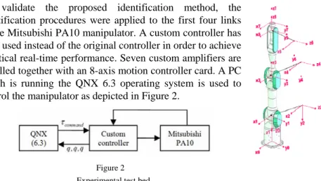
To validate the proposed identification method, the identification procedures were applied to the first four links of the Mitsubishi PA10 manipulator. A custom controller has been used instead of the original controller in order to achieve a critical real-time performance. Seven custom amplifiers are installed together with an 8-axis motion controller card. A PC which is running the QNX 6.3 operating system is used to control the manipulator as depicted in Figure 2.

Figure 2 Experimental test bed

As mentioned above, the following steps were carried out in order to identify the dynamic model:

1 Derive the rigid dynamic model of the robot as in (9) and (10). Noting that the Coriolis-Centrifugal and gravity term is included in this model. Gravity

terms can only be set to zero when robot joints are considered separately as in Section 2.2.

2 Identify the boundary velocity q_thres in which the dynamic friction model becomes linear for each joint (see Table 1 for the experimental results).

Table 1

Boundary velocity for the first four links of the PA10 Joint q_thres(rad s/ )

1 0.25 2 0.27 3 0.3 4 0.6

3 Carry out the optimum exciting trajectory as in Section 2.3. By making use of the Matlab Genetic Algorithm (GA) Toolbox, the optimum trajectory was found with the minimum condition number around 65.

4 Execute the optimum trajectory on the PA10; obtain the joint motion and joint torque data. Note that because the PA10 manipulator does not have joint torque sensor, the joint torques are obtained by measuring the motor currents. An independent joint control scheme is used at each joint to make the joints follow the reference/optimal trajectory.

5 The inertial parameters are estimated using the method as in Section 2.4.

The equivalent virtual parameters as in (16) and (17) are shown in Table 2.

Note that these parameters were obtained with the constraint

(

^{m I,}

)

_i ^>0to

make sure the physical feasibility of the identified results.

Table 2

Virtual parameters X (15) that minimize the cost function (16)

3.2 Model Verification

3.2.1 Torque Reconstruction

As noted in Section 2.2, the result of the above identification process is the parameter h^ˆ_b which is the combination of the base parameters and joint friction coefficients. Since the base parameters are lump from the link inertias h, it is impossible to directly check the correctness of the identified parameters. Instead, the identified model is verified by comparing the reconstructed torques, which are generated from the identified model, and the measured torques, which are the actual joint torques that are used to control the manipulator. Since the major difference between the approach in this paper and others is the use of the boundary velocity, it is necessary to check whether the identified parameters using the boundary velocity has any advantages. To this end, two sets of data have been used to identify h^ˆ_b. The first set (set A) only includes the data points which

have q >q_thres while the second set (set B) includes all the experimental points. In

the case of the PA10 manipulator, the number of data points in set A is about 30%

of the number of data points in set B. Figure 3 shows the measured torques vs. the re-constructed torques of joint 1-4 for an arbitrary and different trajectory in joint space. Motion data ( , , )q q q and joint torque (namely “measured torque”) was recorded. The “re-constructed torque” is then computed as (10). In Figure 3, red represents the measured torque (MT), blue represents the re-constructed torque using h^ˆ_b^B (RTall =W h_{b b}^ˆB) and green represents the re-constructed torque using h^ˆ_b^A (RTthres =W h_{b b}^ˆA). Noting that the time scale for the x-axis is time 10 (ms).

a) Joint 1

b) Joint 2

c) Joint 3

d) Joint 4 Figure 3

Measured torque vs. Re-constructed torque

The root-mean-square (RMS) errors between the measured torque and re- constructed torque are shown in Table 3.

Table 3

RMS errors between the measured and re-constructed torque Joint RT(thres): Set A RT(all): Set B

1 4.1 3.9

2 5.9 7.1

3 1.5 2.1

4 3.7 5.8

Theoretically, one should expect the quality of the identified parameter h^ˆ_b^A using set A is worse than the one using set B h^ˆ_b^B because there are more data in set B.

However, as can be seen in Table 2, an opposite result was obtained. The RMS errors in the first case (set A) are smaller than the second case (set B) for most of the joints. This observation implies that the extra data points in set B contribute negatively to the accuracy of the identified result h^ˆ_b^Bin low velocity regions [9].

3.2.2 Computed Torque Control

Since the purpose of the identification process in this paper is to obtain a model that can be used in advanced model based control schemes, the identified model has been further tested in another experiment as descrbed below:

1 All the joint(s) of the manipulator is commanded to follow a sinusoidal trajectory (amplitude: 30 degree, period = 4s).

2 Two controller schemes were implemented:

a) Independent joint control: no dynamic information was used to compensate for the inertial effects. This control scheme is widely adopted in most industrial manipulator controller because of its simplicity.

b) Dynamic control: the identified dynamic parameters were used. A standard joint space computed control was implemented. The identified dynamic model was used to decouple the dynamic behavior among the axes. Notice that the feed-forward frictions i.e.

the compensated frictions are computed based on the desired joint velocities.

The tracking errors for the first four joints are shown in Figure 4: blue represents the joint tracking errors using the indepedent joint control scheme, red represents the joint tracking errors using the dynamic control.

Figure 4

Joint tracking error comparison between kinematic and dynamic control (left to right, top to bottom:

joint 1 to 4)

It is clear that there is a significant improvement in term of the tracking error for joint 1, 2 and 4. The tracking error for joint 3 is not as much different as others.

One explaination that has been pointed out in [9] is because of the structure of the PA10 that makes the inertial effects at joint 1, 2, 4 are much easier to be excited than the rest of the joints. As a result, the quality of the identified parameters which contribute to the joint torque of joint 3 are poorer. This observation implies that further constraints need to be imposed on the optimum trajectories in order to excite the dynamic effects from different joints evenly.

It is worth pointing that the above identified dynamic model was obtained in the high speed region. Consequently, it is neccessary to see how good the identified model in the low speed region is. In order to check the performance of the identified parameters in the low speed region, the above experiment has been redone with the period of the desired trajectory incresed from 4 s to 40 s. Tracking errors are shown in Figure 5 (blue: indepedent joint control scheme, red: dynamic control).

Figure 5

Joint tracking error (low speed) comparison between kinematic and dynamic control (left to right, top to bottom: joint 1 to 4)

As is seen, the differences between the model based control and non-model based control are no longer significant as in the previous case. One possible explaination is that the inertial effects of the dynamic model has been dominated by joint frictions at low speed region. As a result, the control performance will mainly depend on how joint frictions are compensated in this region.

Conclusions

We have presented a systematic procedure for identification the dynamic model of robot manipulator(s). Two main considerations has been addressed through the process. Firstly, the validity of the most commonly used joint friction model, the combination of viscous and Coulomb friction, was considered. Secondly, the problem of the so-called physical feasibility of the identified parameters has been mentioned. Instead of using the standard linear least-square estimator, a constrained optimization problem was used to obtain the identified parameters.

The proposed approach has been implemented on the first four links of the Mitsubishi PA10 manipulator. The correctness of the identified dynamic model was verified by comparing the reconstructed torques from the identified model and the measured torques from each joint. Furthermore, the usefulness of the identified parameters has also been justified by incorporating the identified dynamic model to the conventional computed-torque control scheme. Significant

improvement in terms of the joint tracking errors was obtained in comparison to the one using non-model control scheme in the high speed region. In the low speed region, however, this observation is no longer true. Thus, a different model should be used to describe the dynamic behavior of the manipulator in this region.

Acknowledgements

The authors would like to thank the members of the Mechatronics group at SIMTech (Singapore Institute of Manufacturing Technology – www.simtech.a- star.edu.sg) who helped conduct the experiment on the PA10 manipulator.

References

[1] An, C. H., C. G. Atkeson, J. M. Hollerbach, Model-based Control of a Robot Manipulator. The MIT Press series in artificial intelligence. 1988, Cambridge, Mass.: MIT Press. p. 233

[2] Khatib, O., A Unified Approach for Motion and Force Control of Robot Manipulators: the Operational Space Formulation. IEEE Journal of Robotics and Automation, 1987. RA-3(1): pp. 43-53

[3] Armstrong, B., et al. The Explicit Dynamic Model and Inertial Parameters of the PUMA 560 Arm. 1986, San Francisco, CA, USA: IEEE Comput. Soc.

Press

[4] Daemi, M., B. Heimann, Separation of Friction and Rigid Body Identification for an Industrial Robot. Courses and Lectures-International Centre For Mechanical Sciences, 1998: pp. 35-42

[5] Armstrong, B., On Finding Exciting Trajectories for Identification Experiments Involving Systems with Nonlinear Dynamics. International Journal of Robotics Research, 1989. 8(6): pp. 28-48

[6] Antonelli, G., F. Caccavale, P. Chiacchio, A Systematic Procedure for the Identification of Dynamic Parameters of Robot Manipulators. Robotica, 1999, 17: pp. 427-35

[7] Grotjahn, M., M. Daemi, B. Heimann. Friction and Rigid Body Identification of Robot Dynamics. 2001, Rio de Janeiro, Brazil: Elsevier [8] Kermani, M. R., R. V. Patel, M. Moallem, Friction Identification and

Compensation in Robotic Manipulators. IEEE Transactions on Instrumentation and Measurement, 2007. 56(6): pp. 2346-2353

[9] Ngoc Dung, V., J. Marcelo H. Ang Jr, Improved Dynamic Identification of Robotic Manipulators in the Linear Region of Dynamic Friction, in the 9^th International IFAC Symposium on Robot Control 2009

[10] Gautier, M., W. Khalil, Direct Calculation of Minimum Set of Inertial Parameters of Serial Robots. IEEE Transactions on Robotics and Automation, 1990, 6(3): pp. 368-373

[11] Gautier, M., Numerical Calculation of the Base Inertial Parameters of Robots. Journal of Robotic Systems, 1991, 8(4): pp. 485-506

[12] Presse, C., M. Gautier. New Criteria of Exciting Trajectories for Robot Identification. 1993, Atlanta, GA, USA: IEEE Comput. Soc. Press

[13] Yoshida, K., W. Khalil, Verification of the Positive Definiteness of the Inertial Matrix of Manipulators Using Base Inertial Parameters.

International Journal of Robotics Research, 2000, 19(5): pp. 498-510 [14] Ngoc Dung, V., J. Marcelo H. Ang, Dynamic Model Identification For

Industrial Manipulator Subject To Advanced Model-based Control, in 4^th International Conference Humanoid, Nanotechnology, Information Technology, Communication and Control, Environment and Management.

2008: Manila, Philippines

[15] Olsen, M. M., J. Swevers, W. Verdonck, Maximum Likelihood Identification of a Dynamic Robot Model: Implementation Issues.

International Journal of Robotics Research, 2002, 21(2): pp. 89-96

[16] Mata, V., et al., Dynamic Parameter Identification in Industrial Robots Considering Physical Feasibility. Advanced Robotics, 2005, 19(1): pp. 101- 19

[17] Khosla, P. K., Categorization of Parameters in the Dynamic Robot Model.

IEEE Transactions on Robotics and Automation, 1989. 5(3): pp. 261-8 [18] Siciliano, B., O. Khatib, Springer Handbook of Robotics. 2007: Springer-

Verlag New York, Inc.

[19] Gautier, M., N. CNRS. Dynamic Identification of Robots with Power Model. 1997

[20] Swevers, J., W. Verdonck, J. De Schutter, Dynamic Model Identification for Industrial Robots. Control Systems Magazine, IEEE, 2007. 27(5): pp.

58-71

[21] Swevers, J., et al., Optimal Robot Excitation and Identification. Robotics and Automation, IEEE Transactions on, 1997, 13(5): pp. 730-740