Determinants of Cost Efficiency: Evidence from Banking Sectors in EU Countries

Determinants of Cost Efficiency: Evidence from Banking Sectors in EU Countries

Jaroslav Belas

¹

, Kristina Kocisova

²

, Beata Gavurova

³

1 Center for Applied Economic Research, Zlin, Faculty of Management and Economics, Tomas Bata University in Zlín, Czech Republic.

E-mail: belas@utb.cz

2 Faculty of Economics, Technical University of Košice. Slovakia.

E-mail: kristina.kocisova@tuke.sk

3 Center for Applied Economic Research, Zlin, Faculty of Management and Economics, Tomas Bata University in Zlín, Czech Republic.

E-mail: gavurova@utb.cz - Corresponding author

Abstract: The purpose of this study was to examine the cost efficiency of banking sectors within the European Union (EU) counties during the period 2008-2017 and to find out which banking sector specific variables and macroeconomic variables influenced cost efficiency. We compared cost efficiency estimated by the traditional model of Data Envelopment Analysis presented by [15] and new cost efficiency model under different unit prices presented by [37] which aimed to make the reader aware of the pros and cons of both methods. Our second stage of analysis included estimation of the regression model in order to find out the determinants of banking sectors´ cost efficiency. Panel data multiple regression was applied to find out the relationship between the depended variable (cost efficiency) and independent variables (banking sector specific variables and macroeconomic variables). Our results showed that cost efficiency was mainly explained by the capitalisation, profitability, loan risk, market structure, conditions of the economy and development of inflation.

Keywords: Data Envelopment Analysis; Cost efficiency; Banking sector; European Union countries

1 Introduction

Research problem. Under the condition of the European Union (EU) countries commercial banks as principal financial intermediaries play an important role in capital allocation. The role is to provide financial intermediation and economic acceleration by converting deposits into productive investment. The role is not only to convert deposits mainly into the loans, but this transformation should be

done with minimal cost. Therefore, it is crucial to study cost efficiency by comparing the transformation process in different banking sectors with different labour costs, interest expenses and other types of costs. In the literature, there are three basic methods through which to measure cost efficiency: the ratio analysis, the parametric approach and the non-parametric approach. The parametric and non-parametric approaches differ primarily in the underlying assumptions applied in estimating cost efficient frontiers. The most commonly employed parametric procedure is the Stochastic Frontier Approach (SFA) as it allows for the effect of statistical noise to be separated from the effect of inefficiency, thereby resulting in a stochastic frontier. However, this approach requires a specific functional form that presupposes the shape of the cost efficiency frontier and assumes a specific probability distribution for the efficiency level. Additionally, if the assumptions are incorrectly specified, the estimated cost efficiency will contain errors. The non-parametric approach, commonly referred to as Data Envelopment Analysis (DEA), avoids this type of specification error because it does not require a priori assumptions about the analytical form of the cost function or an assumed probability distribution for efficiency. However, it has one major drawback in that it does not allow for random errors (e.g. measurement errors, good or bad luck) in the optimisation problem and all deviations from the cost efficiency frontier are marked as inefficiency. As both parametric and non-parametric approaches have their own merits and limitations and as the correct level of cost efficiency is unknown, the choice of a suitable efficiency estimation procedure has been quite controversial [13]. However, in the banking area, some researchers prefer to use parametric method ([40], [17]), while some studies mainly used the non- parametric approach ([20], [25], [19]). We can also find some studies comparing the results of cost efficiency estimated by both methods simultaneously ([41], [24]). Most of the mentioned studies apply the traditional cost frontier to measure efficiency. In modern literature, we can also find some studies dealing with the application of a new cost efficiency function [13], but only a few studies are dealing with the application of this method in the condition of Slovak banking ([32], [42]).

Aim and motivation. Technology and cost are the wheels that drive modern enterprises; some enterprises have an advantage regarding technology and others in cost. Hence, the management is eager to how and to what extent their resources are being effectively and efficiently utilised, compared to other similar enterprises in the same or similar field [10]. Regarding this subject, there are two different situations: one with common unit prices and costs for all Decision-Making Units (DMUs) and the other with different prices and costs from Decision-Making Unit to Decision-Making Unit. Cost efficiency evaluates the ability to produce current outputs at minimal cost. The concept of cost efficiency was first introduced by [15] and then developed by [16] by using linear programming technologies. In this model, it was assumed that input prices are the same across all Decision-Making Units. However, the prevailing price and cost assumption is not always valid in actual business, and it is demonstrated that efficiency measures based on this

assumption can be misleading. So we decided to present a new cost efficiency related model introduced by [37] and compare results obtained by traditional and new cost model. Therefore, in the first stage of the analysis, we applied the DEA model under the condition of variable return to scale to compare traditional and new cost model and then used the more appropriate model to examine cost efficiency within the European Union countries during the period 2008-2017. In the second stage, we aim to examine the determinants of cost efficiency and to find out the relationship between efficiency and banking sectors specific variables and macroeconomic variables. The analysis is realised in a sample of 28 banking sectors based on the data available at the web page of the European Central Bank and Eurostat. The structure of the paper is the following. Section 2 presents a review of the literature on bank efficiency; Section 3 explains the methodology and data used in this paper; while Section 4 presents the results of the analysis.

The last section concludes the paper with a summary of key findings.

2 Literature Review

The analysis of determinants of pricing policy at the bank level in the Czech Republic was examined in the study of [22]. One of the main aims of the study was to evaluate cost efficiency. The authors used DEA and SFA. They pointed to the fact, that cost efficiency is one of the most critical factors of bank pricing policy. The study identified the crisis impact on the behaviour of the banking sector and consequently, on a higher tendency to avoid risk, while the level of flexible response to any changes in interest rate decreased.

During the period 2005-2011 the differences in cost efficiency in six countries of Central and Eastern Europe was examined by [30]. The research was based on the fact that the cost efficiency of banks is inevitable for their stability. The results showed that the macroeconomic stability of a country significantly supported efficiency. The bank with a higher risk profile was considered as more inefficient.

Similarly, the bank with lower liquidity, lower level of solvency and higher credit risk were considered more inefficient than a bank that was more conscious in taking risks. Until 2008, the potential for efficiency increase was evident in the banks of all analysed banking systems. The efficiency decrease was registered in Poland, Romania, Russia and Hungary since 2009. However, the banks in Bulgaria and the Czech Republic noted efficiency stagnation. During the period 2002-2010 cost efficiency of Indonesian banks was researched by [3]. The tendency was decreasing during the examined period. The following factors influenced the cost efficiency of Indonesian banks: bank size, profitability and capital. The positive trend of efficiency is related to the lessons to be learnt by Indonesian banks from the previous crisis during 1997-1998. An adequate environment for management created by the Government of Indonesia resulted in positive performance and cost efficiency measured during the realisation of this study. Also, the authors positively assessed implementation of various programs

that focus on the capital increase in the banks, improvement of competition and efficiency that resulted in a higher bank’s stability to the financial crisis’s impacts during 2007-2008. The most significant determinants of the cost efficiency were the following: inflation rates, the growth rate of the GDP, as well as the unemployment rate. The study provided recommendations for the management of banks in order to more effectively manage banks themselves, increase banks’ sizes regarding assets and capital, manage liquidity and risk, and also provide credits for small business to maintain its credit portfolio. The cost efficiency in the Western European countries was examined by [28]. Authors emphasised numerous changes in the regulatory and competitive environment of banks, including elimination or total removal of trade and entry barriers in these European markets. Also, the authors focused on the need to use the best technologies to create new financial products. The cost efficiency of the European banks was considered crucial. The lack of management skills was regarded as the primary source of inefficiency. Similarly, the technology gap ratio (TGR) that may be interconnected with environmental variables typical of a particular country was a subject of the study. TGR and metafrontier cost efficiency showed a gradual upward trend during 1996-2000. However, the downward trend followed after this period, especially after the subprime mortgage crisis in 2007-2010. The results showed that the competitive banking market influenced higher cost efficiency and reduction of the technology gap in the member states of the EU during 1996-2000.

However, international economic integration was accompanied by an influence of higher risks. The global recession and also the financial crisis affected the evolution of cost efficiency.

The influence of the financial crisis on the banking efficiency in the Euro Area countries was explained by [4]. The result indicated a gradual process of efficiency convergence among the banks of core and peripheral countries until 2008. The financial crisis had an influence on the structure of banking performance during the period 2009-2012. In many cases, the efficiency improved after the crisis that is also related to actual processes of risk management in the banks, processes of lowering costs, and a wide range of monitoring and regulatory processes that had been set in the post-crisis period. The authors highlighted the fact that positive evaluations may be influenced by the misleading interpretation of analytical results about efficiency and may appeal to a necessity of multi- dimensional assessment of efficiency aspects. The impact of financial partnership on efficiency was analysed by [31]. The research focused on Malaysia’s and Islamic banks, their efficiency during 1996-2012, as well as determinants that influenced it. The authors applied SFA. The banks with allocated financial partnership reached higher efficiency than other banks. Similarly, banks with lower capital risk and a higher rate of financial partnership tended to be more efficient. It is necessary to cautiously interpret these results, especially during the period of financial crisis. Governmental authorities agreed that the financial partnership of the banks might represent an efficient strategy in increasing their efficiencies. It is important to evaluate the capital risk of the banks and the rate of their financial partnerships in research and selection of suitable banks for these types of partnerships. The study supported an idea that partnership may be used as

a strategy for improving efficiency, especially due to low capital risk. The competent authorities need to examine the level of partnership as well as capital risk in monitoring banks that offer to finance by a partnership [34]. The DEA method to research banking sector efficiency was preferred by [5]. The main aim was to analyse the efficiency in Turkey and subsequent comparison of participation and conventional banks’ efficiencies. The result indicated that the efficiency of a participation bank was higher than the efficiency of a conventional bank. Both groups of Turkish banks had higher technical efficiency than allocative efficiency. The technical efficiency had a higher impact on cost efficiency. In conclusion, higher allocative efficiency and effective use of resources may increase the cost efficiency in the Turkish banking system. Efficiency and loans represented a positive relationship in forming efficiency determinants. On the other hand, efficiency and expenses, capital, deposit, non-performing loans, bank size, GDP growth and inflation represent a negative relationship especially in the case of conventional banks. Both participation and conventional banks and their efficiency may be influenced by the same determinants differently. The determinants of banking performance about banking indicators, such as ROA, ROE and cost efficiency was examined by [11]. In 2005-2009, 12 banks participated in this research. The result indicated an increase of ROE by 0.06%

and improvement of efficiency by 0.09% by increasing an income diversity of 5%.

The authors deduced that those variables which are connected to government intervention had a negative impact on banks’ performance in conventional banking model. The market share, indicators of population solvency and net credit and total net assets had the most significant influence on ROE. Variables in the DEA model were examined by [36] in order to improve the methodology of efficiency measurement. The idea emerged from methodological procedures’

diversity in measuring banking sector performance. The authors suggested that the banks’ loans and deposits should be used as key variables in the DEA model in order to measure the efficiency of the Lithuanian banks. The authors used the input-oriented DEA model and under the assumption of variable returns to scale.

They concluded that the securities should not be used as a DEA model’s outcome because this variable was not evident as statistically significant in a sample of the Latvian banks. The following inputs were used: deposits from customers, total administrative expense, balances due to credit institutions, equity, interest expense, fees and commission expense, staff expense. The outputs were as follows: loans, securities, net interest margin, operating profit, interest income, fees and commission income. However, the authors did not take into consideration the fact that some variables may be both input and output. In conclusion, the authors stated that it is essential to use such variables that reflect business specificities of all financial market participants in terms of variables’ selection.

The determinants of bank efficiency by DEA models during 2006-2011 was examined by [1]. The conclusion was that cost efficiency was positively affected by market concentration and demand density, while inversely related to branching.

Also, these results were robust to any sample restriction anchored to the distribution of efficiency. Sensitivity analysis highlighted a significant source of cost inefficiency that was related to the risk in local markets. The comparative

analysis, where the meta-regression analysis was used to compare the results from 120 papers published during 2000-2014 was prepared by [2]. The conclusions were following: banking efficiency is lower when parametric methods were used;

value-added approach with intermediation method increased banking efficiency, while hybrid approach lowered it; quality of studies, number of observations and variables determined the level of efficiency; sign and magnitude were different between parametric and non-parametric studies. The Nerlovian Revenue Inefficiency model was applied in the study of [18]. This model enabled to differentiate between technical and allocative inefficiency. As a consequence of this fact, the authors also examined if the inefficiency of banks was caused by technical or allocative inefficiency. The authors suggested researching the influence of the banks’ geographical locations on their total efficiency. The efficiency of the European banks before the crisis, during the crisis and also in the post-crisis period from a technical and allocative efficiency point of view was examined by [39]. The gradual improvement of technical and allocative efficiency was evident, while in a majority of countries in the post-crisis period, the trend of efficiency decrease was notified. The authors used Bayesian dynamic modelling and panel data to analyse the commercial banks that operate in the ‘old’ member states of the EU (15) during 2005-2012. In 2008-2012, there was a decrease in efficiency in the group of large banks. Also, an influence of the lack of banking capital as a consequence of the financial crisis that caused the stagnation of banking credit activities was presented. The authors recommend research of differences between short-term and long-term banking efficiency within the use of dynamic models. The results of [23] are linked to the study mentioned above.

They examined 74 Chinese commercial banks during 2006-2013. The findings showed that banks allocate roughly 59% and 61% of labour and capital, respectively, to collect deposits in the first stage and that the average technical efficiency scores in both production stages were respectively 68% and 84%. The results also support findings that joint-stock banks were the most technically efficient, while larger commercial banks, including the big four state-owned banks, were the least technically efficient. Similar research ambitions were obvious by [13] who examined the consistency of efficiency evaluation results that were obtained by using SFA and DEA methods. Authors used panel data of the Chinese banks during 1994-2007. The results moderated consistency between parametric and non-parametric methods in efficiency rankings, identification of best and worst practice banks, the stability of efficiency over time, and the correlation between frontier efficiency and accounting-based performance measures. The only limitation would be a fact that the Chinese banking sector may be subject to important technological and regulatory processes from a long-term point of view that was not a part of this analysis. Authors appeal to an inevitability of multiple methods’ use at the same time in order to evaluate banking efficiency, and a combination of these methods enable cross-check of the results. Thus, it is possible to reach a more plausible evaluation of the banking sector efficiency.

The primary role of commercial banks is to realise the financial intermediation, i.e. channell of resources from lenders to borrowers with the view to putting the existing assets to best economic use. In European Union countries, a universal

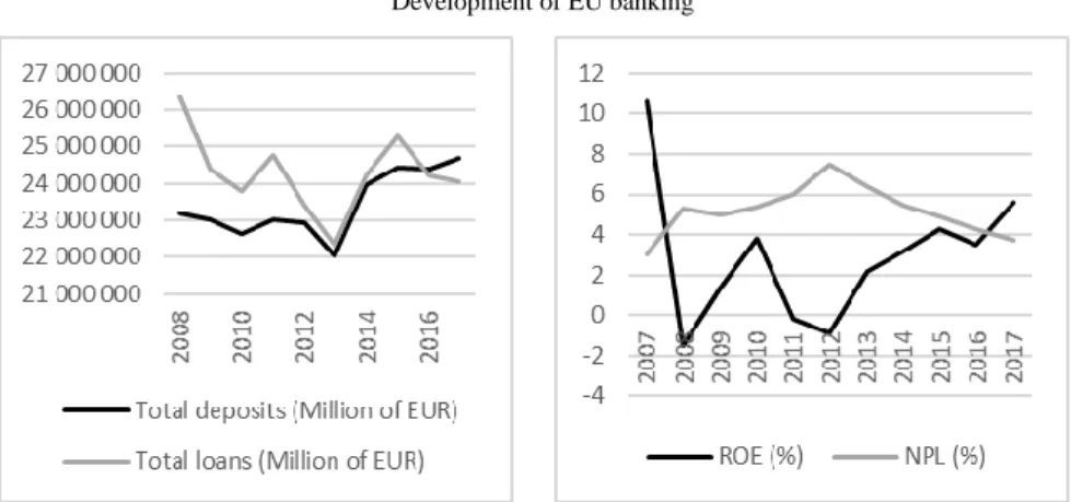
banking model is prevalent. A well-developed financial infrastructure helps citizens save for the future, helps companies borrow to invest and expand, and facilitates the trade of goods and services. The scale of bank´s operations in European Union countries in 2008 was striking: banks managed an equivalent of 144% of EU-27 GDP as loans extended to households and enterprises and held an equivalent of 135% GDP in deposits. During the next year, we can see an increase in deposits and a decrease in loans. In 2017 the total deposit in the EU countries rose to 24.7 trillion EUR, which represents an increase of 6.52% compared to 2008 (Figure 1). This growth was driven by an increase in deposits from households and non-financial corporations. The share of deposit over total assets increased in 2017 to 53.4% from 51.3% in 2016, in line with the rising trend since 2007 when the share of deposit over total assets was 47.3%. That reveals a shift towards greater deposit dependency as a source of funding. The total value of loans outstanding from the EU decreased by 8.67% in 2017 compared to 2008. It was influenced by development between 2008 and 2010 when the total loans decreased by 9.77% due to restriction in loan policy as a consequence of the global financial crisis. After this year the loans started to increase, and the peak was reached in 2015 when the value of total loans in the EU countries was 25.3 trillion EUR (Figure 1).

Figure 1 Development of EU banking

Source: Prepared by the authors The downward trend in the number of EU credit institutions, which started in 2008, continued in all years untill 2017. While in 2008 the number of credit institutions was 8525, in 2017 the number of credit institutions drops to 6250. This trend includes factors such as mergers in the banking sector to enhance profitability. The downward trend can also be seen in case of a number of employees in credit institutions. By end-2017 banks in EU countries employed about 2.71 million people, compared to 3.28 million people in end-2008. The global financial crisis has led to a substantial increase in non-performing loans (NPLs) in banks’ balance sheets. This trend has been increasing since 2008 leading to a maximum NPL ratio of 7.5% in EU countries in 2012 (Figure 1).

However, the NPL ratio trajectories show a significant decline across the EU countries, which can be attributed to increased bank lending activities in recent years. From 2017, the NPL ratio for the EU was only 3.7% suggesting that NPLs are no longer a specific problem of European banks. European banks have continued to build a strong capital position and strengthen their balance sheets.

Capital continued to growth, with Tier 1 ratio in EU banks was 13.8% in 2017. All banks have met the liquidity coverage ratio above the minimum. Also, the leverage and Net stable funding ratio shortfalls continued to decrease. Given that the ECB maintains its ultra-low interest rates, profitability remains a key challenge facing EU banks. The return on equity (ROE), a key indicator for assessing the attractiveness of banking sector for investors is slowly recovering.

The ROE of EU banks was 5.6% in 2017, which represents only half of the values before the outbreak of the financial crisis, but is the highest since 2007 (Figure 1).

The same tendencies can also be seen in the case of ROA [14].

3 Methodology and Data

Data Envelopment Analysis (DEA) was first developed by [8] under the constant return to scale assumption and provides a measure of technical efficiency.

Following [15] and [16], a sequence of linear programmes was applied to construct cost efficiency frontiers, and from these, measures of traditional cost efficiency were calculated. The traditional cost efficiency model assumes that the unit cost of inputs is identical among Decision-Making Units. According to the [32], to be cost-efficient, the Decision-Making Unit must be both technically efficient (adopting the best practice technology) and allocative efficient (selecting the optimal mix of inputs to minimise the costs for a given output).

We define

y

_o as the s1 vector of the o-th production unit´s s outputs )

,..., 1

(r s ^,

x

_o is the

m  1

vector of its m inputs (i1,...,m), Y is the

s  n

matrix of outputs (n denotes the number of DMUs, (j1,...,n)^{), and} X is the

n

m 

matrix of inputs. Let us consider we have prices associated with inputs.

Let c =



c₁,...,c_m



be the standard unit input-price or unit-cost vector. Then the cost efficiency



^{* of} DMU_o is defined as the ratio between minimal the cost and the actual cost:

cxo

cx^*

*

 ⁽¹⁾

Where

x

_o^* is an optimal solution of the constant return to scale cost minimisation DEA model defined in the following terms:

Cost cx cx

x,

*min ⁽²⁾

Subject to xX (3)

 Y

y_o (4)

0

 (5)

The solution to this optimisation problem is known to be the point

x

^* where the isocost line is tangent to the isoquant. This point represents the cost minimising vector of input quantities for the evaluated production unit, given the vector of input prices

c

_o and output levels

y

_o. The isoquant represents all possible combinations of inputs amount



x₁,x₂



that are needed to produce the same amount of a single output. The point x is a point in the interior of the production possibility set representing the activity of a Decision-Making Unit which produces this same amount of output but with a more significant amount of both inputs. To evaluate the performance of this production unit we can use the common Farrell measure of radial efficiency. The result is the measurement of technical efficiency which can be calculated as the ratio between the distance from 0 to

~ x

_and

distance from 0 to x. If the information about the input prices is available, we can also define the isocost line whose slope is given by the ratio of input prices.

Isocost line shows all combinations of inputs which cost the same total amount.

The relative distance of

x ˆ

and

~ x

refers to allocative efficiency which can bring minimal cost but is connected with the loss of technical efficiency [6].

In traditional cost efficiency DEA models, we assume that input prices are the same across all decision-making units. However, real markets do not necessarily function under perfect competition, and unit input prices might not be identical across all Decision-Making Units. Thus, as pointed out by [37] the traditional DEA cost efficiency model does not take account of the fact that costs can be reduced by reducing the input factor prices. For example, if two production units have the same inputs and outputs while the unit input prices for one DMU are twice those of the other DMU, then the total costs of the DMU with the higher unit input prices will be higher than those of the DMU with the lower unit input prices. However, under the traditional DEA model, the cost function is homogeneous of degree one in input prices, and the scaling factor cancels out in the cost efficiency ratio, and thus, the two DMU will be assigned the same measure of cost efficiency irrespective of the fact that they have significantly different input prices. It represents a severe drawback for assessing relative efficiency levels under the traditional DEA model and is caused by the peculiar structure of the DEA model which exclusively focuses on the technical efficiency of two DMU and cannot take account of variations in unit input prices between the DMUs. Therefore, in order to avoid this shortcoming, [37] proposed a new scheme for evaluating cost efficiency under which the production technology is

homogeneous of degree one in the total costs as distinct from being homogeneous of degree one in the input prices under the traditional DEA model. It means that under the new DEA model DMUs with different input prices will return different measures of cost efficiency [13].

The new cost efficiency model is based on the definition of another cost-based production possibility set

P

_c ^{as [10]:}

  

,  ,  , 0



 x y x X y Y 

P_c ⁽⁶⁾

Where X 



x₁,...,x_n



with xj 



c₁jx₁j,...,cmjxmj



^T where (j1,...,n)^{. Here we} assume that the matrices X and C are non-negative, and elements of

 

^{c x}

  

^{i j}



x_ij _{ij ij}  , , where (i1,...,m) ^and (j1,...,n), are denominated in similar units in monetary terms (e.g. euro). The new cost efficiency



^* is defined as [10]:

o o

x e

x e ^*

*

 ⁽⁷⁾

Where

e  R

^m is a row vector with elements being equal to 1, and

x

_o^* is the optimal solution of the linear programmes given below:

New Cost ex ex

o x,

*min ⁽⁸⁾

Subject to xX



₍₉₎

 Y

y_o ₍₁₀₎

0

 ₍₁₁₎

In the new cost efficiency model, the optimal input mix

x

_o^* that produces the output

y

_o can be found independently of the DMU´s current unit price

c

_o, whereas in the traditional cost efficiency model is keeping the unit cost of DMU j fixed at

c

_o we search for optimal input mix

x

^* for producing output

y

_o. These are fundamental differences between the two models. Using traditional cost efficiency model we can fail to recognise the existence of other cheaper input mixes. In our research, we focused on the evaluation of the cost efficiency of EU banking sectors. Banking institutions within the banking sector usually operate under the condition of imperfect competition, financial constraints, regulatory requirements and other factors that do not allow them to operate at their optimal size. For this reason, we used DEA models under the conditions of variable return to scale which minimises the impact of mentioned restrictions. We evaluated the relative efficiency of 28 banking systems during 2008-2017 based on the data available at the website of the European Central Bank (ECB). The term “relative”

efficiency refers to the achieved efficiency of the evaluated banking system within the group of evaluated banking systems and of the criteria used (input and output variables according to the applied approach). We used the intermediation approach to evaluate the cost efficiency of the banking sectors. This approach views the bank as an intermediary of financial services and assumes that banks collect funds (deposits and purchases funds) with the assistance of labour and capital and transform them into loans and other assets. For each banking sector in the sample, it was necessary to select inputs, outputs and input prices. Total deposits and output variables, as well as selected types of costs, are measured in thousands of EUR. We consider two inputs, namely, total deposits (x1), and the number of employees (x2). Each of these inputs generates costs, referred to total interest expenses, and staff costs. Therefore, we can easily calculate prices for each input as a ratio of the particular cost to the selected input. The price of deposits (c1) can be calculated as the ratio of total interest expenses to total deposits, and the price of labour (c2) as the ratio of staff costs to the number of employees. On the output side, we consider two types of outputs: total loans (y1) and other earning assets (y2), which refer to non-lending activities. We provide descriptive statistics of all input, output variables and input prices in selected years used to calculate efficiencies in Table 1. The calculations of cost efficiency were done using the R software [33]. In the process of calculation of cost efficiency all input, output variables, and input prices were put together in one dataset. The reason for putting data together is that we would like to eliminate the change of efficiency affected by the change due to the technological progress, which could lead to the shift of the efficiency frontier. Within the second stage of the analysis, in order to examine the internal (banking sector specific variables) and external (macroeconomic) factors that affect the cost efficiency of banking sectors in EU countries, the following model has been developed:

it L

l lYlit J

j jXjit

CEit   

 

 



1 ,

1 ,

(12)

CEit is the cost efficiency of the banking sector i at time t, with i = 1,…,N; and t = 1,…,T; Xj,it is the banking sector specific variables of bank i at time t, with j = 1,…,J; and Yj,it is the macroeconomic variables with l = 1,…,L; and ɛit is the disturbance. To examine the determinants of cost efficiency, we selected the independent variables, which has been used in most studies on bank efficiency.

We can divide the independent variables into two groups: the banking sector specific variables and macroeconomic variables. As a banking sector, specific variables were used: total equity over the total assets (capitalisation), net interest margin, total loans to total assets, and cost to income ratio. We used the ratio of total equity to total assets (ETA) to measure the capital strength of the banking sector. In general, we assume that a higher capital ratio indicates higher safe in the banking sector. To determine a relationship in case of this variable is not entirely clear. One point of view is that capital ratio is expected to have a positive sign since we assumed that banks are predicted to be rewarded with additional

revenues for holding the optimal amount of capital ([27], [20]). The second point of view says that capital ratio is expected to have a negative sign since it is assumed that banks which hold the higher value of capital cannot provide these funds in the form of loans and this way reduces the value of potential interest income ([38], [26]). We used the net interest margin (NIM) as the profitability indicator. We can expect that more cost-efficient banking sectors can earn a higher profit, which should lead to a positive relationship between NIM and cost efficiency. The existence of a positive relationship was described for example in the work of [32] and [3]. We used the share of total loans over the total assets (TLTA) as the indicator of credit risk. As the loans are the primary item on the bank´s balance sheet, we can expect that increasing share of loans on the total assets indicate a higher probability of clients´ default and this way higher risk of bank failure. The higher share of problematic loans can lead to additional cost, and therefore we can assume a negative relationship between the TLTA and cost efficiency. The existence of a negative relationship was described, for example, in the works of [21] and [35]. The cost to income ratio (CI) as the indicator of operating efficiency represents the share of operating costs to operating income.

Decreasing value of this indicator suggests that banks use their resources rationally and effectively. Therefore, we expect a negative relationship between CI and cost efficiency.

Table 1

Descriptive statistics on variables used for efficiency measurement in selected years

Variable 2008 2011 2014 2017

Total deposits (thousands of EUR)

Minimum 22529538 16204830 18391566 20990278 Maximum 4825242292 4365091099 5165173780 4964894562 Average 828314461 823053108 856281966 882280472 St.dev. 1247055577 1254404587 1390576096 1431605287 Number of employees

Minimum 3872 4026 4426 4920

Maximum 685550 663800 649900 597319

Average 117192 110695 101976 96812

St.dev. 170551 162459 153096 143242

Price of deposits

Minimum 0.0291 0.0148 0.0034 0.0026

Maximum 0.2433 0.0808 0.0462 0.0351

Average 0.0616 0.0331 0.0189 0.0118

St.dev. 0.0385 0.0144 0.0088 0.0075

Price of labour (thousands of EUR)

Minimum 108.54 109.22 121.98 133.83

Maximum 1606.20 1576.59 1697.62 1937.94

Average 679.00 705.00 704.71 742.91

St.dev. 433.27 466.09 487.17 496.59

Total loans (thousands of EUR)

Minimum 25494424 15165481 16146218 14612609 Maximum 5109275497 4729262760 4687794919 4286872201 Average 941490575 885183481 865485292 859829418 St.dev. 1443001244 1339990410 1346364169 1333638597 Other earnings assets

(thousands of EUR)

Minimum 1499987 988552 1340534 645256

Maximum 3879104144 5874885874 5364815194 3117402948 Average 500810288 554052432 505773886 339879781 St.dev. 1007846235 1243601727 1133071099 705709326 Cost to income ratio

Minimum 0.4050 0.3124 0.3695 0.4064

Maximum 1.8618 0.7213 0.7256 0.7402

Average 0.6300 0.5624 0.5650 0.5665

St.dev. 0.2673 0.0934 0.0876 0.0788

Total equity to total assets

Minimum 0.0293 -0.0059 0.0411 0.0528

Maximum 0.1402 0.1945 0.1511 0.1508

Average 0.0629 0.0738 0.0855 0.0912

St.dev. 0.0266 0.0405 0.0289 0.0276

Net interest margin

Minimum 0.0079 0.0058 0.0067 0.0046

Maximum 0.0473 0.0477 0.0411 0.0337

Average 0.0210 0.0217 0.0208 0.0190

St.dev. 0.0107 0.0116 0.0094 0.0082

Total loans to total assets

Minimum 0.4720 0.3573 0.3850 0.4302

Maximum 0.9634 0.8612 0.7663 0.7648

Average 0.6970 0.6615 0.6441 0.6493

St.dev. 0.1193 0.1260 0.0852 0.0794

Herfindahl-Hirschman index

Minimum 0.0191 0.0317 0.0300 0.0250

Maximum 0.3490 0.3880 0.3630 0.2419

Average 0.1136 0.1112 0.1150 0.1145

St.dev. 0.0775 0.0758 0.0747 0.0622

Index of a gross domestic product

Minimum 102.40 89.40 80.80 81.40

Maximum 126.90 132.50 141.10 165.20

Average 111.73 109.26 112.54 124.34

St.dev. 6.72 8.86 13.19 19.56

The harmonised index of consumer prices

Minimum 78.33 92.43 98.84 99.45

Maximum 99.50 102.36 101.57 104.48

Average 89.75 95.72 100.09 101.90

St.dev. 3.95 2.20 0.62 1.35

Source: Prepared by the authors In addition to the banking sector, specific variables the analysis included a set of macroeconomic variables like an indicator of market structure, real gross domestic product, and inflation. The market structure in the banking industry is usually measured by the Herfindahl-Hirschman index (HHI). The increasing value of HHI indicates that the level of competition in the banking sector decreases and the market power is concentrated in the hand of the biggest banks on the market. In our study, we expect a positive relationship between the bank concentration ratio and cost efficiency, which is in line with the traditional structure-conduct- performance paradigm. In a highly concentrated market, enterprises have higher market power which allows them to set prices above marginal costs and achieve higher efficiency. Higher concentration reduces competition by fostering collusive behaviour among firms, whether more concentrated market improves market performance as a whole. Index of gross domestic product (GDP) reflects the conditions of the economy. We assume that the growing economy will provide a growing demand for banking services and lower risk; therefore, we expect a positive relation with cost efficiency. According to [12] the effect of inflation on efficiency depends on whether wages and other operating expenses increase faster than inflation. Many studies ([7], [29]) have found a positive relationship between inflation and cost efficiency. However, if inflation is not anticipated and banks do not adjust their interest rates correctly, there is the possibility that costs may increase faster than revenues and hence affect bank efficiency negatively. Inflation is measured by the Harmonised index of consumer prices (HICP). We present the descriptive statistics of all banking sector specific variables and macroeconomic variables in selected years in Table 1. In order to examine the determinants of EU banking sectors´ cost efficiency, we applied the regression analysis for panel data.

Model (1) was estimated through a pooling regression taking each banking sector´s cost efficiency (CE) as the dependent variable. The opportunity to use a panel structure of the data frame was tested with the Chow test. If the p-value of the Chow test is lower than 0.05 at 95% significance level, then it is suitable to use a panel structure of the model. A precondition for the use of a linear model is stationarity of time series. In the literature, there are several tests of stationarity of time series. To verify the stationarity in the case of our sample, we used the augmented Dickey-Fuller test (ADF test). If the data are stationary, it allows us to analyse the relationship between variables through a linear model. Primary and most used method for estimating the parameters of a linear model (regression coefficients) is the ordinary least squares method (OLS). The normality of residues distributions was tested by Lilliefors (Kolmogorov-Smirnov) normality test. The presence of the heteroscedasticity by the Goldfeld-Quandt test. To verify the correlation between the independent variables was used VIF test.

4 Results and Discussion

At first, we want to demonstrate the difference between traditional and new cost efficiency model with a simple example involving 28 banking sectors in 2017 with each using two inputs

 x

1

, x

2



to produce two outputs

 y

1

, y

2



along with input costs

 c

₁

,c

₂



. The data and the resulting measurement are exhibited in Table 2. For the banking sector in Netherland, the traditional cost model gives the efficiency score



^*

 1

. The traditional cost model assumes that the unit cost of inputs is identical among, so do not take into account the actual prices of production units.

Table 2

Comparison of traditional and new cost efficiency

x1 x2 c1 c2 y1 y2 x1 x₂ e₁ e2 _{Cost Cost}

Austria 683563615 71927 0.0097 897.97 668211550 159978945 6638108 64588090 1 1 0.4475 0.4880 Belgium 736069787 53002 0.0159 1270.92 663830236 191132030 11694628 67361120 1 1 0.5842 0.4368 Bulgaria 43339685 30070 0.0046 133.83 31444887 7197650 199209 4024320 1 1 0.1547 0.5004 Cyprus 60280326 10632 0.0151 528.24 43345469 4814871 913225 5616260 1 1 0.4415 0.4171 Czech

Republic 212269639 41566 0.0056 392.57 201357569 30748224 1183177 16317680 1 1 0.2939 0.6185 Germany 4643112339 597319 0.0126 757.27 4151780258 1828168231 58549722 452333000 1 1 0.4763 0.4176 Denmark 277901421 42240 0.0237 770.58 635571192 159863483 6591714 32549240 1 1 0.8472 0.8452 Estonia 20990278 4920 0.0030 385.08 18857486 645256 63361 1894600 1 1 0.8057 0.7499 Spain 2573541252 183016 0.0153 1591.53 2298517928 684184706 39425041 291274830 1 1 0.6363 0.3578 Finland 288022396 20999 0.0085 819.08 273029377 47404295 2441404 17199900 1 1 0.6636 0.7381 France 4013514129 398516 0.0209 1431.96 4218882008 1594188332 84004911 570659000 1 1 0.6994 0.3311 United

Kingdom 4964894562 353299 0.0104 1348.42 4286872201 3117402948 51721425 476394970 1 1 0.8287 0.5233 Greece 212619376 41707 0.0103 550.81 177600789 30243587 2196832 22972700 1 1 0.2750 0.3816

Croatia 51008131 20434 0.0113 303.50 41854113 8465001 575900 6201750 1 1 0.2535 0.3906 Hungary 100176994 38877 0.0066 307.08 71914285 34218858 656250 11938500 1 1 0.1681 0.3325 Ireland 275382985 26891 0.0106 1131.33 262388042 95891662 2913747 30422600 1 1 0.5166 0.4185 Italy 1853534489 281928 0.0103 943.47 1893333371 547181303 19089514 265989930 1 1 0.3420 0.3422 Lithuania 24320392 8922 0.0030 187.73 19175587 1510252 73834 1674930 1 1 0.4655 0.8490 Luxembourg 622719094 26149 0.0113 1451.17 477274000 137463504 7062961 37946750 1 1 0.7943 0.5547 Latvia 24126954 8492 0.0058 352.39 14612609 4996593 141073 2992480 1 1 0.4890 0.4979 Malta 40027646 4924 0.0188 436.36 24568413 17566753 752613 2148630 1 1 0.8492 0.8245 Netherlands 1550227495 75215 0.0351 1937.94 1825197654 325947293 54435385 145761970 1 1 1.0000 0.4699 Poland 310320217 168800 0.0139 187.03 290719709 106852515 4300291 31570810 1 1 0.1530 0.4294 Portugal 306306111 46238 0.0114 687.94 241657251 85870011 3488864 31809000 1 1 0.3080 0.3652 Romania 80598771 55044 0.0059 204.32 55812592 19855043 475572 11246680 1 1 0.1091 0.2869 Sweden 637987857 70877 0.0239 1078.36 1101745032 254319209 15258667 76430780 1 1 0.7906 0.6214 Slovenia 35453871 9844 0.0037 434.23 26490120 9294822 131151 4274560 1 1 0.4057 0.4428 Slovakia 61543416 18879 0.0026 280.36 59179989 11228503 159229 5292980 1 1 0.2815 0.6484 Source: Prepared by the authors The new scheme devised as in [37] distinguishes banking sectors by according them different cost efficiency scores. This is due to the difference in their unit costs. We can see the drop in Netherland banking sector from one

 

^*Netherland



to 0.4699

 

^*Netherland



. Its higher cost structure explains this drop in banking sector performance. We can see that banking sector in Netherland uses 1550227495 thousand of EUR of input 1 (total deposits) with a price of 0.0351 EUR per one unit of deposits and 75215 persons of input 2 (number of employees) with a price of 1937,94 thousand of EUR per one employee. When we look at the unit cost in different banking sectors, we can see that unit cost was the highest. Therefore the banking sector in the Netherlands could not be considered as cost-efficient. It indicates that all banking sectors that use the same amount of inputs to produce the same amount of outputs but take into account different unit prices then the total costs of the banking sectors are different. Therefore we could not consider them the same cost-efficient. Therefore, we decided to analyse the cost efficiency of the banking sectors in EU countries under the new scheme described by [37].

Following the described methodology we evaluate the new cost efficiency of banking sectors within the EU countries during 2008-2017. As it was mentioned above, the intermediation approach was applied. According to the intermediation approach the input and output variables, and their prices, for each banking sector were defined. Table 3 shows the development of new cost efficiency in individual EU banking sectors and average values for the whole EU banking sector during 2008-2017. We observed no dramatic changes in the average new cost efficiency during the analysed period, but we can see notable differences among the observed countries. Table 3 shows the results of an average new cost efficiency obtained relative to the whole sample during the analysed period. The minimum average value was reached in 2008, the maximum average value in 2014. Results showed that the average new cost efficiency increased from 39.88% in 2008 to 53.31% in 2014 and then decreased to 51% in 2017. The average new cost efficiency at the beginning of the analysed period was 39.88% indicating that on average, banking sectors could save 62.12% of their costs by using the inputs in

optimal combination while maintaining the given input prices. On average the European banking sector did not use the minimum amount of inputs for producing the given outputs, and the proportion of inputs did not guarantee the minimum possible costs. At the end of the analysed period, the average new cost efficiency was 51%, indicating potential cost-saving equal to 49%. The results of analysis per country, indicate that the new cost efficiency ranged from 14.45% (in Belgium in 2008) to 100%. The highest scores were recorded in countries like Germany (2011), Estonia (2014), the United Kingdom (2011, 2014 and 2015), Ireland (2011), and Malta (2014). The lowest scores were observed in countries like Belgium (2008, and 2009), Hungary (2012 and 2013), and Romania (2010, 2011, 2014, 2015, 2016 and 2017). Improvement in new cost efficiency during the analysed period can be seen in Austria, Belgium, Bulgaria, Cyprus, Czech Republic, Denmark, Estonia, Finland, Greece, Hungary, Italy, Lithuania, Luxembourg, Latvia, Malta, Netherlands, Poland, Portugal, Romania, Sweden, Slovenia and Slovakia. The decline in new cost efficiency can be seen in Germany, Spain, France, the United Kingdom, and Ireland. The most significant decrease between the years 2008 and 2017 occurred in Germany, where the new cost efficiency decreased from 86.30% to 41.769%. On the other hand, the highest increase was recorded in Belgium, where the new cost efficiency increased from 14.45% to 43.68%. The result of the analysis can suggest different banking behaviour for specific countries. Therefore, in the second stage, the regression analysis with a set of banking sector specific variables and macroeconomic variables will be done.

Table 3

New cost efficiency of the EU banking sectors, 2008-2017

2008 2009 2010 2011 2012 2013 2014 2015 2016 2017

Austria 0.3624 0.4146 0.4360 0.4340 0.4296 0.4330 0.4680 0.4680 0.4493 0.4880 Belgium 0.1445 0.1788 0.3036 0.2871 0.3133 0.3670 0.3768 0.3978 0.4228 0.4368 Bulgaria 0.4176 0.4226 0.4342 0.4341 0.4290 0.4468 0.4576 0.4410 0.4772 0.5004 Cyprus 0.3998 0.4001 0.3923 0.3593 0.3634 0.3570 0.4564 0.4809 0.3911 0.4171 Czech Republic 0.3361 0.3488 0.3595 0.3553 0.3538 0.3955 0.4198 0.4329 0.4819 0.6185 Germany 0.8630 0.6763 0.6613 1 0.7642 0.6596 0.7016 0.6902 0.4991 0.4176 Denmark 0.4133 0.4331 0.5171 0.4861 0.5055 0.5264 0.6358 0.6497 0.6701 0.8452 Estonia 0.4887 0.5882 0.6435 0.5847 0.7591 0.7721 1 0.9566 0.9491 0.7499 Spain 0.3693 0.4059 0.4178 0.3837 0.3732 0.3478 0.3530 0.3770 0.3680 0.3578 Finland 0.4790 0.4776 0.6615 0.8440 0.7171 0.6642 0.8445 0.7129 0.7446 0.7381 France 0.3693 0.2985 0.2989 0.3066 0.3028 0.3075 0.3194 0.3171 0.3337 0.3311 United Kingdom 0.6292 0.6972 0.7791 1 0.8332 0.6594 1 1 0.6028 0.5233 Greece 0.2820 0.3071 0.3192 0.2856 0.2916 0.2797 0.3232 0.3428 0.3731 0.3816 Croatia 0.3916 0.3882 0.3848 0.3814 0.3779 0.4061 0.3943 0.3876 0.3885 0.3906 Hungary 0.2357 0.2298 0.2280 0.2387 0.1954 0.1964 0.3324 0.3242 0.2869 0.3325 Ireland 0.6124 0.7004 0.8124 1 0.8322 0.9568 0.4928 0.4838 0.4133 0.4185 Italy 0.2657 0.2892 0.2995 0.2915 0.2956 0.2952 0.3020 0.3137 0.3035 0.3422 Lithuania 0.5208 0.5671 0.6109 0.6751 0.7215 0.7318 0.7103 0.7625 0.8115 0.8490 Luxembourg 0.3489 0.5304 0.7173 0.6210 0.6716 0.7326 0.6848 0.6383 0.6215 0.5547 Latvia 0.4448 0.5049 0.5637 0.5976 0.6172 0.6130 0.6121 0.6143 0.5063 0.4979 Malta 0.6044 0.7792 0.8806 0.8626 0.9112 0.9978 1 0.8362 0.8377 0.8245 Netherlands 0.2990 0.3529 0.3793 0.3732 0.3922 0.4141 0.4133 0.4454 0.4569 0.4699 Poland 0.2311 0.2374 0.2475 0.2711 0.2584 0.2801 0.4060 0.4089 0.4592 0.4294

Portugal 0.3054 0.3561 0.3655 0.3408 0.3496 0.3463 0.3646 0.3365 0.3829 0.3652 Romania 0.1918 0.1896 0.2136 0.2171 0.2152 0.2248 0.2394 0.2512 0.2743 0.2869 Sweden 0.3390 0.4356 0.4493 0.4705 0.5226 0.5908 0.6501 0.6681 0.6406 0.6214 Slovenia 0.3788 0.4224 0.4310 0.4060 0.3980 0.3751 0.5181 0.5231 0.4455 0.4428 Slovakia 0.4439 0.4270 0.4495 0.4279 0.4281 0.4467 0.4509 0.4735 0.6048 0.6484 Minimum 0.1445 0.1788 0.2136 0.2171 0.1954 0.1964 0.2394 0.2512 0.2743 0.2869 Maximum 0.8630 0.7792 0.8806 1.0000 0.9112 0.9978 1.0000 1.0000 0.9491 0.8490 Average 0.3988 0.4307 0.4735 0.4977 0.4865 0.4937 0.5331 0.5262 0.5070 0.5100 St.dev. 0.1511 0.1564 0.1837 0.2410 0.2094 0.2124 0.2200 0.1980 0.1736 0.1658 Source: Prepared by the authors To explain the variability in new cost efficiencies, we regressed the new cost efficiencies (CE) on the set of relevant banking sector specific variables and macroeconomic variables. The testing of the model was implemented in program R. The opportunity to use a panel structure of the data frame was tested with the Chow test. The proposed model (12) was tested for statistical significance of the model (F-statistics). The normality of residues distributions was tested by Lilliefors (Kolmogorov-Smirnov) normality test. The presence of the heteroscedasticity by the Goldfeld-Quandt test, and the multicollinearity by the VIF test.

Table 4

Determinants of new cost efficiency

Coefficient t-statistics p-value

Cost to income ratio (CI) -0.02061 -0.5284 0.5976703

Total equity to total assets (ETA) 1.596 4.3704 0.000018 ***

Net interest margin (NIM) -10.197 -9.1985 < 2.2e-16 ***

Total loans to total assets (TLTA) -0.30635 -3.4010 0.000772 ***

HHI index (HHI) 0.66848 4.9918 0.000001 ***

GDP index (GDP) 0.0024755 3.3602 0.00089 ***

Inflation (HICP) 0.0044088 4.2337 0.000031***

Sample size Balanced Panel: n=28, T=10, N=280

R² (Adjusted R²) 0.37556 (0.36184)

F-statistics F-statistics: 23.4277 on 7 and 273 DF, p-value: < 2.22e-16 Chow Test F = 5.6295, df1 = 637, df2 = 1700, p-value < 2.2e-16

ADF test stationary

Lilliefors normality test D = 0.05637, p-value = 0.03161

Goldfeld-Quandt test GQ = 0.69277, df1 = 133, df2 = 133, p-value = 0.9824 VIF test CI (1.1009); ETA (1.8609); NIM (1.9271); TLTA (1.3187);

HHI (1.1386); GDP (1.2903); HICP (1.1234)

‘***’ 0.01 ‘**’ 0.05 ‘*’ 0.1

Source: Prepared by the authors Table 4 reports the regression results for our models. As can be seen, there was no problem with heteroscedasticity, and multicollinearity and the residues were normally distributed. Six variables were identified as the statistically significant:

capitalisation, profitability, loan risk, market structure, conditions of the economy and inflation. The capitalisation measured as the ratio of total equity and total assets had positive and significant, similar to the findings of [20], [27], [32], or [31], and [3], who assumed that banks are predicted to be rewarded with