VISCOSITY RELATIONSHIPS FOR POLYMERS IN BULK AND IN CONCENTRATED SOLUTION

VISCOSITY RELATIONSHIPS FOR POLYMERS IN BULK AND IN CONCENTRATED SOLUTION

T. G Fox, Serge Graten, and S. Loshaek

I. Introduction 431 II. Experimental 432

1. Theoretical Considerations 432 2. Viscometric Techniques 434

a. Pipette- and Capillary-Type Viscometers 435

b. Tensile-Creep Measurements 437 3. Preparation and Characterization of the Polymer Sample 439

III. Empirical Viscosity Relationships 440 1. The Molecular-Weight Dependence for Long Chains 442

2. Viscosity-Temperature Relationships for Polymers in Bulk 446

3. Combined η-Τ-Μ Relationships 456 4. The Effect of Molecular-Weight Heterogeneity 457

5. The Effect of Branching 459 6. The Viscosity of Concentrated Solutions of Polymer Chains 459

a. Viscosity-Temperature Relationships 461 b. The Isothermal Dependence on Polymer Chain Length 462

c. Isothermal Viscosity-Concentration Relationships 463

IV. Molecular Theories of Flow 466

1. Historical 466 2. Early Theories of Flow 467

3. The Eyring Theory of Flow 469 4. The Flow Mechanism for Polymer Chains 471

5. The Isothermal Dependence of Viscosity on Chain Length 472

6. The Theoretical Calculation of / 477 7. Free Volume and the Jumping Frequency 480

8. Semiempirical Equations 484 9. Non-Newtonian Behavior 488

Nomenclature 492 I. Introduction

The need for knowledge of the factors influencing the nonrecoverable flow of high polymers in bulk and in concentrated solution and for a molecular interpretation of these relationships has increased with the technological advances in recent years. In order to gain a satisfactory under- standing of flow, extensive data are required on well-defined polymers over wide ranges in the important variables of molecular weight, M; tempera- ture, T\ and diluent type and concentration. Substantial progress has been

431

made in the last decade with the advent of such data for a variety of poly- mers, from which useful empirical laws and a quantitative molecular picture of flow were deduced.

The purpose of this chapter will be (1) to point out the experimental problems which arise and the methods which have been utilized for their solution, (2) to review the available data and to establish empirical laws of flow which are generally applicable and which fall within the framework of existing molecular concepts, and (3) to interpret the results in terms of qualitative and quantitative molecular theories of flow.

We shall consider here the viscosities of bulk polymers and of polymer- diluent systems wherein the concentration of the diluent is not sufficient to separate the coiled polymer chains to an extent where they behave as a set of hydrodynamically interacting but otherwise independent units, i.e., we shall not be concerned with the properties of very dilute solutions. We shall refer to the coefficient of resistance to flow in shear simply as the viscosity.

We shall avoid the use of the terms melt viscosity and bulk viscosity for this purpose since the former refers only to the viscosity of crystalline poly- mers above their melting points, and the latter has been used in the past to designate the coefficient of the resistance to shrinkage in compression.

II. Experimental

Many precautions must be taken in order to obtain reliable viscosity data over wide ranges of molecular weight, temperature, and diluent type and concentration. These are necessary because of complications arising from the superposition of time-dependent elastic (recoverable) deformations on the viscous (nonrecoverable) flow, and deviation above some critical shear rate of the rate of shear-shear stress dependence from Newtonian behavior.

Of course, it is necessary to use well-characterized samples and to ensure that the experimental conditions are such as to prevent these samples from changing during the measurement. Since reliable viscosity data can be obtained only if these problems are recognized, we shall discuss them briefly in the following sections.

1. THEORETICAL CONSIDERATIONS

The complications which arise in measuring the viscosity of a liquid polymer can be demonstrated clearly by a consideration of the deformation processes which occur when the sample is subjected to a constant tensile load. For this purpose we shall briefly review the currently accepted picture of the molecular mechanisms involved.¹

In a bulk (undiluted) sample of an amorphous unoriented linear polymer or in a concentrated solution of such a polymer, each flexible long-chain

1 F. Bueche, J. Appl. Phys. 26, 738 (1955).

molecule assumes a random configuration in space such that the average distribution of the chain segments of a given molecule about its center of gravity is Gaussian or nearly so. These randomly coiled molecules are closely packed so that the domains of neighboring molecules in the liquid overlap and one molecular chain is intimately enmeshed in the complicated web of polymer chains spun by its neighbors. The result is that the polymer chains are entangled, much like a pile of entangled ropes.

When a force is applied to such a system, deformations occur by four dif- ferent processes which take place simultaneously. The first of these is a relatively small elastic (completely recoverable) deformation which reaches its maximum steady value in a very short time, and which corresponds to the distortion of primary and secondary valence bonds. Such a response is exhibited by crystalline solids as well as liquids. The second process con- sists of a time-dependent elastic deformation which approaches asymptoti- cally an equilibrium value that can be calculated from the concentration of chain entanglements by the methods of the well-known kinetic theory of rubberlike elasticity.²'³ Here we assume that the polymer system acts like a cross-linked network with the entanglement points between neighboring chains representing the network junctures. Since the entanglements are not permanent, however, the entanglement points will slip past each other after a period of time and eventually the system will behave as though the network structure does not exist. During this period both a time- dependent elastic deformation and an unrecoverable viscous flow will occur. The former represents the stretching (uncoiling) under the influence of the external force of the individual polymer chains (in accordance with the theory of Kuhn⁴) to an upper limit predictable from the stress and the molecular weight of the chains. The permanent viscous deformation, on the other hand, represents the slipping of molecular chains past each other and continues to take place at a rate which, in the simplest case at least, is proportional to the applied stress.

In isolating the viscous deformation, advantage can be taken of the fact that the elastic deformations approach limiting values whereas the viscous deformation does not; consequently, at sufficiently long times the former contribute only a negligible portion of the total deformation. Since the time scale of these changes is considerably shortened with either increas- ing temperature or increasing diluent concentration, at high temperatures or diluent concentrations the elastic deformations reach their equilibrium values in a very short time and substantially all of the deformation at

2 L. R. G. Treloar, "The Physics of Rubber Elasticity," Oxford, New York, 1949.

3 P. J. Flory, "Principles of Polymer Chemistry," p. 464. Cornell U. P., Ithaca, N. Y., 1953.

4 W. Kuhn, Kollid-Z. 68, 2 (1934); 76, 258 (1936).

reasonable times represents viscous flow. Under these conditions viscosity measurements can be made by simply ignoring the negligibly small elastic effects. At low temperatures and low diluent concentrations, however, most of the deformation in a reasonable period of time will be elastic, and it becomes necessary to employ relatively long periods of time in order to observe and separate the viscous and elastic components of flow. Methods for accomplishing this are discussed below in a description of tensile creep measurements.

Another complication which presents itself is the dependence of the vis- cosity on the rate of shear. At low shear rates the flow of an amorphous liquid polymer may be defined in terms of the rate of shear dy/dt and the applied stress r by Newton's law

dy __ r dt η

where the proportionality constant η is the Newtonian viscosity. At higher rates of shear, however, this simple Newtonian behavior is not observed but, instead, the more general relation

applies. In this case the apparent viscosity coefficient calculated from (dy/dt)/r decreases as (dy/dt) increases. A theoretical treatment of this effect in satisfactory agreement with available experimental data has been given by Bueche.⁵ According to his result, Newtonian behavior will pre- vail providing the rate of shear is appreciably lower than a critical value, namely, the characteristic natural frequency of oscillation (stretching and compression) of the coiled polymer chain as it rotates about its center of gravity in the viscous medium. Thus, it is possible to obtain η either by working at very low shearing stresses and shearing rates, or by employing suitable theoretical or empirical means for extrapolating to such conditions.

2. VISCOMETRIC TECHNIQUES

In Table I we have listed some of the methods which have been used suc- cessfully for measuring Newtonian viscosity.

I t is desirable for any instrument to combine as many as possible of the following features: simplicity of construction and operation, a wide operat- ing range of viscosities, a small sample requirement, ease of thermostating over a wide temperature range, a means of providing an inert atmosphere over the sample to prevent degradation, availability of wide range of shear stresses and shear rates, and the possibility of obtaining the combined elastic and viscous response of the material in a single operation. No single

6 F. Bueche, J. Chem. Phys. 22, 1570 (1954).

10-2-10³ 1-10⁵ 1-10⁶ 10³-10⁸ 10M0⁹ lOMO¹¹ 10³-10¹⁰ 10³-10¹² 10^δ->10^{2 5}

6 7 6, 8α,6

9α, b 10

8α 11 12 1 TABLE I

SUMMARY OF METHODS FOR MEASURING VISCOSITIES

Useful Viscosity

Method Range (poise) (approx.) Ref.

Capillary Pipette Falling Sphere

Uniform Bore Capillary Capillary Extrusion Parallel-Plate Plastometer Falling Coaxial Cylinder Stress Relaxation Rotating Cylinder Tensile Creep

instrument listed in Table I combines all of these features; therefore it is usually necessary to compromise on one or more instruments on the basis of the experimental variables being investigated. In many investigations where more than one method has been employed to cover a wide range of conditions, the equivalence of different methods in the overlap region has been demonstrated, in some cases by different workers.¹· *. βα, n, 13, M

Because of the extremely simple experimental techniques and apparatus and small sample requirements of the capillary-tube viscometer and tensile-creep methods, together with the very wide range of applicability afforded by the combination of these methods, we shall very briefly describe their use. A description of many of the useful instruments and techniques has been given elsewhere by Doolittle.¹⁵

a. Pipette- and Capillary-Type Viscometers^ßtS·^16α

Pipette-type viscometers consisting of a Pyrex capillary tube (of 0.5 to 0.8-mm. bore and about 25-cm. length) having at a convenient point along

6 P. J. Flory, J. Am. Chem. Soc. 62, 1057 (1940).

7 J. D. Ferry, E. L. Foster, G. V. Browning, and W. M. Sawyer, / . Colloid Sei. 6, 377 (1951).

8« T. G Fox and P. J. Flory, J. Am. Chem. Soc. 70, 2384 (1948).

* T. G Fox and P. J. Flory, / . Phys. Chem. 55, 221 (1951).

9* R. S. Spencer and R. E. Dillon, J. Colloid Sei. 3, 163 (1948).

96 R. S. Spencer and R. E. Dillon, J. Colloid Sei. 4, 241 (1949).

10 G. J. Dienes and H. F. Klemm, J. Appl. Phys. 17, 458 (1946).

11 R. D. Andrews and A. V. Tobolsky, / . Polymer Sei. 7, 221 (1951).

12 R. Buchdahl, J. Colloid Sei. 3, 87 (1948).

13 J. D. Ferry and G. S. Parks, Physics 6, 356 (1935).

14 G. J. Dienes and F. D. Dexter, J. Colloid Sei. 3,181 (1948).

16 A. K. Doolittle, "The Technology of Solvents and Plasticizers," p. 743. Wiley, New York, 1954.

" · T. G Fox and P. J. Flory, / . Appl. Phys. 21, 581 (1950).

166 T Q γοχ a n (j p j Flory, / . Polymer Sei. 14, 315 (1954).

the tube a small bulb (0.2- to 4.0-cc. capacity) with marks above and below the bulb have been used for measurement of viscosities from 0.01 to 1000 poises. For viscosities from 1 to 10⁶ poises, straight precision-bore Pyrex capillary tube viscometers (1.0- to 2.0-mm. bore and about 25 cm. long), marked at two or more points along the tube have also been used exten- sively. For both types, the relation between the absolute viscosity, η (in poises), the applied pressure differential, P (in millimeters of mercury), and the time, t, (in seconds) for flow betw^reen two marks is given by

η = cPt

Here c is a calibration constant which can be accurately determined from the tP product of a standard fluid, or in the case of the straight tube viscometer it may be calculated from the capillary dimensions and the equation deduced from Poiseuille's law

= 106σ

C Ä2² - Ai²

where σ is the cross-sectional area (in square centimeters) and A2 and hi are the distances (in centimeters) of the lower and upper marks, respec- tively, from the lower end of the tube.

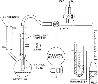
FIG. 1. Schematic diagram of apparatus for measuring viscosities with the capil- lary pipette viscometer.

A convenient apparatus for measuring viscosities by this method is illustrated in Fig. 1. The sample (ca. 1 or 2 gm.) is placed in a Pyrex tube

(ca. 15 cm. long and of 1-cm. internal diameter), which is in turn sur- rounded by a constant boiling vapor bath or other thermbstated bath.

Prior to heating, with the viscometer far above the surface of the sample, the air is evacuated from the system and replaced by an inert atmosphere of nitrogen. The sample is then heated as high above its softening tempera- ture as possible without causing degradation. The upper stopcock is then turned alternately to vacuum and nitrogen until the cessation of the evolution of gas bubbles indicates that the sample is free of volatile impuri- ties. At this point a coherent bubble-free mass of polymer should be present at the bottom of the sample tube with a nitrogen atmosphere over it in readiness for making a viscosity measurement. The measurement of viscosi- ties greater than about 105 poises may be very difficult or impossible by this method, because the time required for the polymer sample to flow down the sides of the tube and form a coherent mass is impractical, or is so long that degradation of the polymer will occur in the meantime.

To proceed with a measurement, the flow of nitrogen gas through the"

capillary is stopped λνΐπΐβ the lower end of the viscometer is immersed in the liquid polymer. After the viscometer has reached the temperature of the system, a reduced pressure (ca. 2 to 20 cm. below atmospheric pressure) is applied by turning the lower three-way stopcock to connect the viscometer with the pressure reservoir, which is of sufficient size (about 1 liter) to elimi- nate pressure surges during the course of the measurement. The time re- quired for the polymer to flow up between two successive marks is deter- mined. The average pressure differential is read on the mercury manometer and corrected for the mean difference in height between the polymer in the viscometer and the surrounding polymer. Immediately after the run the stopcocks are turned to admit nitrogen to the capillary which causes the viscometer to empty slowly.

For polymers mixed with volatile diluents the loss of solvent during a measurement can be minimized if the pressure differential is obtained not by employing a vacuum but, instead, by applying a positive pressure to the surface of the polymer through the side arm of the sample tube.

It is advisable to carry out at least two determinations in each case as a check on the precision. With the straight capillary-tube viscometer this is accomplished most conveniently by timing the flow between successive pairs of marks on the capillary. Values of η obtained with these viscometers are generally reproducible to ± 3 % .

b. Tensile-Creep Measurements

The tensile-creep method is particularly useful for the measurement of very high viscosities (105 to 1025 poises) since it affords a simple technique

for separating the elastic and viscous components of deformation. The technique which is described here is essentially that given by Bueche.1

The optimum size sample will be dictated by the viscoelastic properties of the polymer and the rates of shear employed. A convenient size specimen may be 10 cm. long, 1.5 cm. wide, and 0.05 cm. thick. Such samples may be prepared by casting a solution of the polymer in a volatile solvent onto a mercury surface. Care must be taken, however, to remove all traces of this solvent by heating under vacuum for adequate times.

A simple test chamber which fits conveniently into a thermostated bath consists of a glass cylinder of about 75-mm. diameter and 30-cm. length, sealed off at one end. The sample is clamped at both ends and one of the clamps is anchored to the bottom of the cylinder, while the other is at- tached to a wire which passes through a one-holed stopper in the top of the cylinder and thence over a pulley. The tensile force is applied to the sample by hanging weights from a hook at the end of this wire. A desiccant placed in the bottom of the cylinder serves to keep the humidity in the chamber low. The elongation of the sample is measured as a function of time by observing the motion of an ink mark on the sample or the motion of one of the clamps with a sensitive cathetometer. Before starting any measurements the sample should be conditioned (a day or more) while being held in place in the test chamber at the highest temperature at which meas- urements are to be taken. This procedure tends to eliminate, for some poly- mers at least, the effect of the history of the sample. To avoid complications resulting from changes in the cross-sectional area, it is desirable that over-all elongations greater than about 10% should be avoided.

To obtain a viscosity value by this method, it is necessary to determine a creep curve (change in length, AL, vs. time, t, both measured from the moment of application of the load) for times sufficiently long that a meas- urable component of the deformation is nonrecoverable flow, and then to remove the load and determine the recovery curve (both AL and t being measured from the moment the load was removed).

One may calculate the viscosity by two methods from the data thus ob- tained. The most reliable method is to plot the difference (AL') between the elongation in the creep and recovery curves against time. The viscosity can then be calculated from the slope of the straight line thus obtained by the equation

_ Vs(F/A)

η d(AL'/L)/dt

where F/A is the tensile force per unit cross-sectional area, L is the initial unstretched length of the sample, and the factor of l^ is used to convert tensile viscosity to ordinary shear viscosity.

A second method is to allow the sample to recover as completely as it will. For an experiment where after application of the load for time t and after complete relaxation the nonrecoverable elongation was ΔΖ/', one has

_ V3(F/A)

" (ΔΖ/'/D/i

3. PREPARATION AND CHARACTERIZATION OF THE POLYMER SAMPLE

Since it is generally desired to establish a relationship between the vis- cosity, its temperature coefficient, and the average chain length of a poly- mer, it is extremely important that the polymer be well characterized with respect to molecular weight. We shall see later that the viscosity and its temperature coefficient depend on different molecular weight averages, e.g., the η-Τ coefficient depends on the number-average (Mn) molecular weight whereas, above a certain limiting molecular weight at least, the isothermal viscosity depends on the weight-average (Mw) molecular weight.

It is therefore desirable to know at least these two averages for the members of the homologous series under investigation. It is necessary to measure only one of these when the molecular-weight distribution is known as, for example, from previous studies of the kinetics of polymerization or where polymer fractions are employed wherein the ratio Mw/Mn = 1.

Because the value of Mn and hence of the ψ Τ coefficient is particularly sensitive to the presence of low molecular weight material, special pre- cautions must be taken to remove residual monomer or solvents from the polymer. This can generally be accomplished by evacuating the sample at an elevated temperature (ca. 180 to 217° for polystyrene¹⁶). The speed of outgassing is increased with an increase in temperature and a decrease in sample thickness. For samples having η > 10⁶ poises at the degassing temperature, effective outgassing may be possible only for very thin films.¹⁷ If the impurity is nonvolatile, the polymer may be dissolved in and pre- cipitated from a volatile solvent which can then be more readily removed.

Precautions should also be taken to ensure the stability of the polymer sample under the conditions of measurement⁸·¹⁶ since thermal and oxidative degradation and/or cross-linking reactions may occur which affect the structure and molecular weight of the polymer with a concomitant effect on the viscosity. Such complications may be avoided or minimized by (1) rigorously excluding oxygen from the system, particularly at high tempera- tures, (2) adding a stabilizer to the polymer (e.g., 0.5% of phenyl-ß-naph- thylamine greatly retards the degradation of polystyrene at elevated tem- peratures), and (3) preparing the polymer with relatively stable end groups (e.g., the thermal polymerization of styrene in diethylbenzene yields

" N. Grassie, J. Polymer Sei. 6, 643 (1951).

a more heat-stable polymer than a comparable polymer prepared by bulk polymerization with benzoyl peroxide). The occurrence of degradation may be readily detected by changes in the viscosity after repeated measurements at the same temperature at various time intervals or more directly and pre- cisely by measuring the molecular weight of the polymer before and after a viscosity measurement.

In carrying out viscosity measurements on polymer-diluent systems it is essential that the diluent be homogeneously dispersed and its concentration accurately known. It is desirable, Avhere possible, to determine the concen- tration of the diluent in the mixture by a chemical or physical analytical method. Techniques for preparing homogeneous polymer-diluent samples involving diluents of various degrees of volatility have been described.¹ ·¹⁸·¹⁹ Here it may also be necessary to show that the concentration of diluent did not change appreciably during the measurement.

III. Empirical Viscosity Relationships

In presenting the empirical viscosity relationships we shall be concerned with those which are based, at least qualitatively, on existing molecular concepts of flow, and at the same time are capable of reproducing with reasonable accuracy the viscosity behavior of a wide variety of polymers.

These may be regarded as useful approximations both to the observed data and to more accurate theoretical forms which are not precisely defined at present, and thus contribute to an understanding of the mechanism of flow.

We shall not be concerned with equations which are intended primarily to reproduce accurately observed data without regard to the theoretical sig- nificance of the form of the relationship or the parameters therein.

We shall therefore employ the generally accepted theory of flow as a guide in representing the observed data. Although this theory will be discussed more thoroughly in a subsequent section, it will be useful to summarize its important features here. According to this picture, the primary process of flow for a long-chain molecule enmeshed in a molecular snarl with its neighbors is the activated jump over an energy barrier of a small section or segment of the chain from one position to another in the liquid. The motions of the individual segments are not completely independent, how- ever, since they are joined by valence bonds into molecular chains, which in turn may be entangled with each other into a network structure. It is thus postulated that the viscosity can be expressed as the product of the reciprocal of the jump frequency, J, at which a segment jumps from one position to another, and a statistical factor, F, expressing the requirement

18 T. G Fox and A. R. Shultz, unpublished results.

19 F. Bueche, J. Appl. Phys. 24, 423 (1953).

that the motions of the segments be coordinated, i.e., F

' - 7

It is reasonable to expect that the segmental jump frequency J will be dependent on temperature, and for a given substance presumably on the local configurational arrangement of nearest neighbor polymer segments about a given segment in the liquid. The latter dependence may be ex- pressed in terms of a free volume, φ, associated with this local configura- tional structure. While we shall postpone any discussion of an exact defini- tion of φ until a subsequent section, it presumably should depend on the temperature, (number-average) chain length, Zn , and diluent type and concentration (wi).

On the other hand, the coordination factor, F, is postulated to be inde- pendent of the temperature and of the free volume, and to depend on the (weight-average) number of atoms in the chain (Zw). Thus equation (1) may be expressed more explicitly as

F(ZW)

J(T, Φ) (la)

Since F(ZW) is postulated to be temperature-independent, the dependence of J(T, φ) on T, Zn , and Wi can be determined from the effect of these vari- ables on the viscosity-temperature coefficient. The nature of F(ZW) can then be determined separately from η-Ζ data obtained at fixed temperature and diluent concentration. In practice this is simplest for long chains since for these it is observed that at a given temperature φ and J(T, φ) are independ- ent of Z.

In the succeeding sections we shall discuss first the empirical isothermal viscosity-molecular weight relationships for long chains which lead to an evaluation of F(ZW). We will then discuss η- Τ relationships which shed light on the effect of T, Zn , and W\ on segmental mobility. Finally, we will con- sider data on the effects of molecular-weight heterogeneity, branching, and diluent type and concentration.

The weight-average and number-average chain lengths are defined by the usual equations, i.e.,

Zw = Σν)χΖχ

and

>~=m'

where wx is the weight fraction of species x having a chain length (number of chain atoms) of Zx .

1. T H E MOLECULAR-WEIGHT DEPENDENCE FOR LONG CHAINS

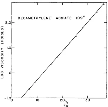
Prior to 1940 the investigations of viscosity-molecular weight relation- ships were confined chiefly to low values of the latter (M < 1000).¹⁵ In that year Flory⁶ reported the results of accurate viscosity determinations on molten linear polyesters (e.g., decamethylene adipate) of known molecular weight and molecular-weight distribution. He found that over the unusually broad ranges in molecular weight (200 to 10,000) and temperature (0 to 200° C.) which were investigated, the data were represented accurately by the relation

log v = CZtl² + A (2)

which is illustrated in Fig. 2. Here C is a constant and A is temperature- dependent. By measuring viscosities of mixtures of polyesters of widely differing molecular weights, Flory was able to show that equation (2) was applicable to any molecular-weight distribution provided the weight- average chain length was used therein.

Although no claim was made originally for the general applicability of equation (2), for a number of years it was applied to data on various poly- mers in bulk and in solution. Perusal of those various sets of results⁸⁰ re- veals, however, that the molecular-weight range covered usually was too

2.0 ω

UJ

</)

S a.

>_ 1.0 (/) O O (/)

>

e> o o

H' ° 0 10 20 _(/ 30

7²

FIG. 2. Illustrative example of Flory's⁶ data on polyesters.

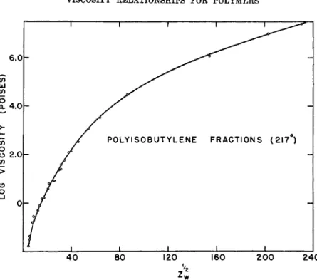
2 4 0

FIG. 3. The nonlinear dependence of log η on ZU² for polyisobutylene.⁸ limited to provide a significant test of its applicability, or that the molecular weights were determined by methods which fail to yield an accurate measure of the weight-average chain length or of something consistently propor- tional to it.

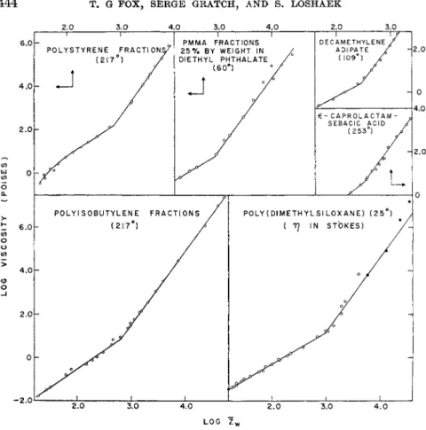
Evidence that equation (2) does not apply universally to other polymers was provided by viscosity data on fractionated polymers of polyisobutylene⁸ and of polystyrene.⁸⁰'¹⁶ As illustrated for polyisobutylene in Fig. 3, plots of log η vs. Z^U2 are not linear for either of these polymers over the wide range in the molecular weight investigated. Instead, excepting for the lower molecular-weight fractions, the data in both cases^{8 a}·^{9 &}·^u·^{1 6}'^{2 0} when plotted on log-log plots (Fig. 4) of η vs. Z are represented by straight lines of identical slope, corresponding to the relation

log v = 3.4 log Zw + K (3) where K is a function of temperature. By measuring viscosities of mixtures of fractions it was shown that the weight-average chain length was the pertinent average applicable in this case.

More recently, viscosity measurements on concentrated solutions of H. Leaderman, R. G. Smith, and R. W. Jones, J. Polymer Sei. 14, 47 (1954).

FIG. 4. Plots of log η vs. log Zw for polymers of different types including poly- styrene,¹⁶⁶ poly (methyl methacrylate),¹ decamethylene adipate,⁶ e-caprolactam- sebacic acid,²⁶ polyisobutylene,⁸ and poly (dimethyl siloxane).²³ The dark circles for poly (dimethyl siloxane) represent viscosity values in poises for a slightly differ- ent temperature (43° C.).²³⁶·^c

polystyrene,¹⁹ polyisobutylene,²¹ and of polymethyl methacrylate¹ over a wide range in temperature and concentration show that, at fixed concen- ration of diluent and fixed temperature, the viscosity is proportional to Zw just as in equation (3),^{3 , 4} except below a certain critical chain length Zc, where approximate proportionality to a lower power of Z is observed.

The value of Zc for a given polymer series varies inversely as the concentra- tion of polymer in solution, i.e., for a given type of polymer the product v2Zc is constant,^1,19 where v2 is the volume fraction of polymer in solution.

It is noteworthy that equation (3) applies to at least three dissimilar polymers both in bulk and in concentrated solution, over extremely wide

21 M. F. Johnson, W. W. Evans, I. Jordan, and J. D. Ferry, J. Colloid Sei. 7, 498 (1952).

ranges in Zw , i.e., at least 87-fold for polyisobutylene and tenfold for poly- styrene. Furthermore, failure of this equation was not observed even for the highest molecular weight investigated but instead occurred only below some relatively low critical chain length Zc, where Zc < 1000 for bulk polymers. This failure at a low chain length, whose value for a poly- mer series depends inversely on the polymer concentration, suggests some abrupt change in the mechanism of flow when the domains of the chains fail to overlap to some critical extent.

It is clear from the experimental results that equation (2) cannot be made to represent the data on polyisobutylene or polystyrene, even in the low molecular weight range for which it is valid for polyesters. In view of the above remarks, we should consider whether equation (3) is applicable to the polyester data, particularly in the high molecular weight range.

We have, therefore, reexamined on isothermal plots of log η vs. log Zw

all of the available viscosity data which cover wide molecular-weight ranges for well-characterized polymers. As illustrated by typical examples in Fig. 4, the data in each case can be represented by two lines which inter- sect at a value of the chain length which we shall call Zc. For chains longer than this critical length, the data covering a wide range of temperature and polymer concentrations in most cases may be represented within the ex- perimental uncertainties in Z and 77 by a straight line of slope 3.4. Thus the data on polyesters which have heretofore been represented by equation (2) are also represented adequately by equation (3).

We have summarized in Table I I the systems for which data are avail- able which conform to equation (3). It is evident that we must regard this equation as an empirical law of flow which may be expected to hold gener- ally for long flexible chain molecules in bulk or in solution.

The dependence of the values of K in equation (3) on temperature and on concentration and the molecular-weight dependence of η for chains shorter than the critical length will be discussed in subsequent sections.

Anticipating the discussion in the theoretical section, a molecular flow theory^22a has been developed by F. Bueche, which predicts a viscosity-mo- lecular weight dependence for long chains in semiquantitative agreement with equation (3). The theory also predicts an abrupt change in the mo- lecular-weight dependence at a critical chain length below which the chains are too short to form a network structure through chain entangle- ments. According to this, the generalization illustrated in Table II that the value of Zc is lower for the more polar polymers is reasonable since the higher forces in this case should result in a higher concentration of chain entanglements than in the nonpolar case.

22e F. Bueche, J. Chem. Phys. 20, 1959 (1952).

T A B L E I I

A P P L I C A B I L I T Y O F T H E E M P I R I C A L L A W log η — 3.4 log Zw + K TO L O N G P O L Y M E R C H A I N S

Range of Applicability

Polymers [Polymer]} viZc at Highest Z Temp, range and mol.

wt. fraction break* studied studied, ° C. wt. detm'n]

Polymer solvent pair

Polyisobutylene⁸ Polyisobutylene-xylene²¹ Polyisobutylene-decalin²¹ Polystyrene¹⁶

Polystyrene-diethyl ben- zene¹⁹

Poly (dimethylsiloxane)²³

Poly (methylmethacryl- ate)-diethyl phthal- ate¹

Decamethylene sebacate⁶ Decamethylene adipate⁶ Decamethylene succinate⁶ Diethylene adipate⁶ ω-hydroxy undecanoate²⁴

Poly(e-caprolactam) :²⁵ linear

tetrachain octachain

Linear Nonpolar Polymers 1.0 610 0.05-0.20 ~1400 0.05-0.20 —

1.0 730 0.14-0.44 ~1000

1.0 —950 53,000 140,000 140,000 7,300 22,500 34,000 Linear Polar Polymers

0.25 208

1.0 290 1.0 280 1.0 290 1.0 290 1.0 <326

24,000

960 1,320 990 1,190 1,443 Effect of Branching 1.0 324 1.0 390 1.0 550 2,300 1,560 2,000

- 9 to 217 25 25 130 to 217

30 to 100 25

60

80 to 200 80 to 200 80 to 200 0 to 200

90

253 253 253

/:(*) W&f:M W&f:(_v) f:(v) /:(*)

WITT, L.S.

/:(*)

W:E W:E W'.E W:E W\E

W'.E W'.E W'.E

* Z_c is t h e lowest chain length for which e q u a t i o n (3) is valid for t h e solution wherein vi is t h e volume fraction of p o l y m e r .

t / = fraction, W = whole polymer. Chain lengths d e t e r m i n e d from η = intrinsic viscosity, π = osmotic p r e s s u r e , L . S . = light s c a t t e r i n g d a t a , E = end group a n a l y s i s .

2. VISCOSITY-TEMPERATURE RELATIONSHIPS FOR POLYMERS IN BULK

The complexity even for simple liquids of viscosity-temperature rela- tionships is evidenced by the large number of empirical expressions for this

226 F . Bueche, J. Chem. Phys. 2 1 , 1850 (1953).

23a A. J . B a r r y , / . Appl. Phys. 17,1020 (1946).

236 M . J . H u n t e r , E . L. Warrick, J . F . H y d e , and C. C. C u r r i e , J. Am. Chem. Soc.

68, 2284 (1946).

23c E . L . Warrick, W. A. Piccoli, and F . S t a r k , unpublished r e s u l t s .

24 W. O. B a k e r , C. S. Fuller, a n d J . H . Heiss, / . Am. Chem. Soc. 6 3 , 2142 (1941).

25 J . R . Schaefgen a n d P . J . Flory, J. Am. Chem. Soc. 70, 2709 (1948).

dependence which have appeared in the last 40 years.¹⁵ The most generally accepted of these is the well-known Andrade equation²⁶

η = const. e^E,RT (4)

More recently an equation of this form was developed by application of the absolute rate theory to the process of flow.²⁷ In this theory the constant E = Rd In η/ά(1/Τ) is identified as the activation energy for the primary process of flow, i.e., for the jump of a small molecule or of a segment of a polymer chain from one equilibrium position in the liquid to the next.

Close scrutiny of actual data reveals, however, that in many cases equa- tion (4) does not apply except over relatively narrow temperature ranges;²⁸ i.e., plots of log η vs. \/T over wide temperature ranges are not linear as required by this equation. The observed deviations are particularly large for polymer chains in bulk and in concentrated solutions.

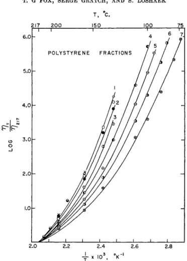
The complexity of the η-Τ relations for a liquid polymer is illustrated in Fig. 5 where data for ten polystyrene fractions of molecular weight from 1675 to 134,000 and temperatures from 217 to as low as 75° are plotted as log (ητ/η2π) vs. l/T⁷.⁸«·¹⁶⁶ The viscosity ratio is employed in order to eliminate from consideration the isothermal dependence on F(Z) discussed in the previous section. The data are represented by curves, whose slopes increase markedly with decreasing temperature. The data for all fractions above 19,000 fall on a single curve (curve 1) whereas for shorter chains a series of curves are obtained, their slopes at a given temperature being lower the lower the chain length. Clearly the viscosity-temperature coefficient depends both on the temperature and, below a certain chain length, on the degree of polymerization.

A clue to the origin of this behavior is furnished by equation (1). Dif- ferentiation of that expression yields the result

*- - ^R [mh] - Awm] ^m

As explained previously, J depends explicitly on temperature T and on free volume φ. Since the latter also depends on temperature, we obtain for a bulk polymer of chain length Z

It appears that the first term in equation (lc) may indeed represent an ac- tivation energy in the sense of the absolute rate theory of flow; the second

26 E. N. da C. Andrade, Nature 125, 309, 582 (1930); Endeavour 13, 117 (1954).

27 S. Glasstone, K. J. Laidler, and H. Eyring, "Theory of Rate Processes," p.

477 ff. McGraw-Hill, New York, 1941.

M R. H. Ewell, / . Appl. Phys. 9, 252 (1938).

T, °C

217 200 150 100 75.

6.0

5.0

4.0

P* R

o

2.0

1.0

■ ^ I ■ ■ ■ ■ ■ ■ ■

2.0 2.2 2.4 2.6 2.8 - f x I0³, ·Κ"'

FIG. 5. Nonlinear dependence of log ητ/vm on 1/Τ^8α· ^16δ Curve 1: fractions of M ^ 19,300. Curves 2-7: fractions of M = 13,300, 6650, 3590, 2600, 2085, 1675, respec- tively.

term, however, is of a completely different nature, representing as it does, the effect of the change of free volume with temperature. Thus, somewhat naively, we may suppose that viscosity changes with temperature through two distinct effects: the first represents the increased energy available at higher temperatures to the individual segments to overcome potential barriers against jumps; the second represents the greater free volume avail- able at higher temperatures, which greater free volume should decrease the potential barriers against jumps.

Unfortunately our knowledge of the character of the terms appearing in equation (lc) is not sufficient to employ it to predict accurately the ob- served viscosity-temperature relationships. However, with reasonable

T⁶ 490⁶ '

2.0

ΡΊΡ*

I I I I Γ POLYSTYRENE / FRACTIONS

J L

10 20 30

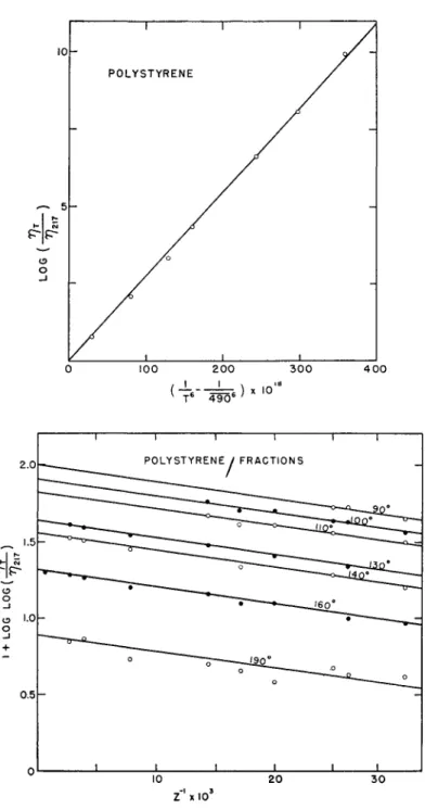
FIG. 6. Representation of data on polystyrene fractions¹⁶⁶ according to equation (6).

Hio.o

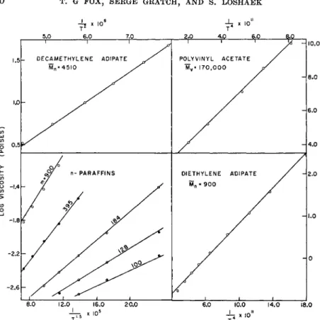
FIG. 7. Representation of data on various polymers⁶·^{3 0}-^{3 1} according to equation (6).

assumptions about the terms in this equation and the dependence²⁹ of φ on T and Zn , we can show that an equation of the form

1 r£a (5)

should serve as a useful practical empirical approximation to the actual behavior. Integration of this equation yields an expression for ητ , i.e.,

log W * r i ) = ^Β\τψϊ ~ j i p ) < ^~ßlZn (6) In these equations, α, β, B, and B' are constants whose values may depend on the polymer.

Empirical equations of the form of equations (5) and (6) have been re- ported to apply over wide ranges in T and Z for fractions of both poly- styrene¹⁶⁶ and polyisobutylene.⁸⁶ The fit of the data for polystyrene by equa-

29 T. G Fox and S. Loshaek, J. Polymer Sei. 16, 371 (1955).

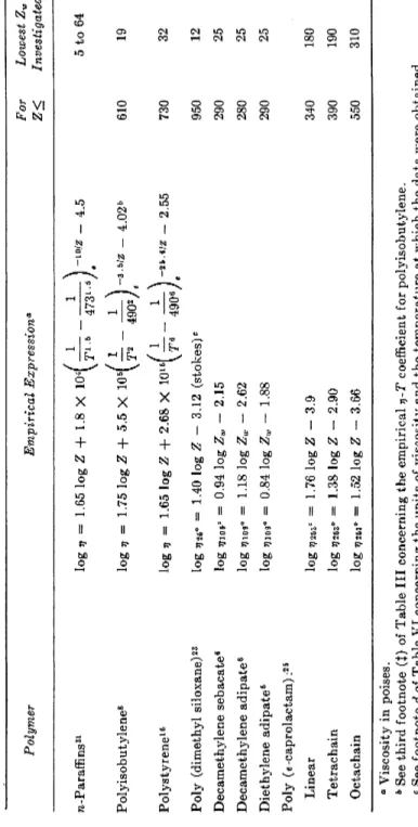
TABLE I I I

VISCOSITY-TEMPERATURE RELATIONSHIPS TOR LINEAR POLYMER CHAINS

ET = (B/T«)e-f»^z

Polymer Poly (methyl methacryl-

ate)¹ * Polystyrene¹⁶⁰· ^b Polyvinyl acetate³⁰ * Diethylene adipate⁶ * Decamethylene adi-

pate⁶ * Polyisobutylene⁸ n-paraffins³¹ *

a 12 5 3 3 1 1 0.5

B 2.7 X 10³⁶ 7.4 X 10¹⁷ 1.8 X 10¹² 3.8 X 10¹¹ 3.1 X 10⁶ 5.06 X 10⁶ί 1.25 X 10*

ß

25.6

3.5J 10

Maximum range investigated Temperature

(°C.) 110 to 150°

75 to 217°

60 to 200°

0 to 167°

82 to 202°

-40 to 217°

-10 to 300°

No. Chain atoms, Z 1380 to 90,000

32 to 2,600 3950

285f 54f

19 to 44,000 5 to 64

* These empirical relationships were derived by the present authors from the pub- lished tabulation of the original data.

t Data given for polyesters¹ of other molecular weights were presented only graph- ically in the original publication, hence no attempt was made to fit them to the equa- tion presented here.

t These constants for polyisobutylene represent our estimate of the "best values"

obtained when all of the reliable data covering the widest range in both T and Zn are considered. They differ slightly from corresponding values published elsewhere.⁸⁶·²⁰ tion (6) is illustrated in Fig. (6), where plots of log-log (ητ/vm) vs. 1/Z for various temperatures are represented by a set of parallel straight lines, whose intercepts when plotted as log (ητ/mu) vs. [ l / Γ⁶ — (1/490⁶)] are linear. In this case the values of a and ß thus determined empirically are 5 and 25.6, respectively. Similar treatment of the data for polyisobutylene fractions yields corresponding values of 1 and 3.5 for these constants.

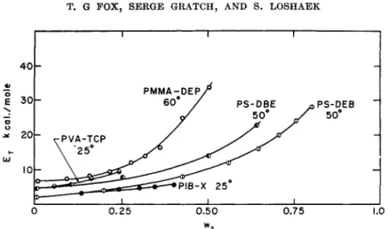
Examination of the existing viscosity-temperature data on seven poly- mers varying greatly in structure demonstrates that they can be represented to a satisfactory approximation by equations (5) and (6). The nature of the agreement is illustrated in Fig. 7, where typical results for several polymers are shown. The parameters obtained for the various polymers are sum- marized in Table III, and in Tables VI and VII where the combined vis- cosity-molecular weight-temperature relationships are given.

It is noteworthy that the values of a in Table III are larger the higher the glass temperature of the polymer. Presumably high polarity or steric hindrance to rotation about the primary valence bond results in both a

30 R. J. Kokes and F. A. Long, / . Am. Chem. Soc. 75, 6142 (1953).

31 A. K. Doolittle, J. Appl. Phys. 22, 1031 (1951).

higher value for Tg and a more severe dependence of the viscosity on temperature.

Since the last paragraph was written a highly useful and suggestive em- pirical representation of the segmental mobility which does, in fact, relate the viscosity-temperature coefficient to a single parameter, the glass tem- perature, has been proposed by Williams³²" and discussed in greater detail by Williams, Landel, and Ferry.³²⁶ The important parameter in their rela- tion is the ratio aT = ηΤ8ρ8/η8Τρ, where η and p are the viscosity and density at temperature T and η8 and p8 are the corresponding quantities at T8. In place of viscosities the ratio of mechanical or electrical relaxation times may be used. They found that a plot of log aT against T-T8 with a suitable choice of T8 gives a single composite curve for all of the data for a wide variety of polymers, polymer solutions, and organic and inorganic glass forming liquids over a temperature range of T8 ± 50°, i.e., aT is a uni- versal function in this temperature range. The relationship is expressed accurately by

η_τ_ __ - 8 . 8 6 ( Γ - Γ . )

[0g

VTs (101.6 + T-T8) ^{u ;}

The small variation of the pT factor has been neglected.

The values of the constants in the equation and the values of T8 for the various systems are dependent on an arbitrary choice of T8 for one system.

This was taken originally as 243° K. for polyisobutylene. Values of T8 thus determined for various substances are reported to lie about 50° above the corresponding glass temperatures (Table IV). If this approximation is ac- cepted, it follows from equation (7) that

ητ -17.44(Γ-Γ,)

l 0 g

^⁼( 5 1 . 6 + T-r.) ^{( 7 α )}

If T8-TQ is not 50° in each case, the value of the constants in this equation will vary slightly from one substance to the next. Ignoring this possibility, equation (7a) relates the viscosity-temperature coefficient of a polymeric system to a single parameter—its glass temperature, which is known for a large number of polymers or may be readily measured. In practice, how- ever, T8-Tg is usually not exactly equal to 50°, and a better fit of the observed behavior is obtained with equation (7).

Differentiation of equation (7) yields the result

E* = ⁴·^{1 2 X 1Q8}(101.6 +T-T.V ^{( 8 )}

32« M. L. Williams, J. Phys. Chem. 59, 95 (1955).

3²⁶ M. L. Williams, R. F. Landel, and J. D. Ferry, J. Am. Chem. Soc. 77,3701 (1955).

T A B L E IV

V I S C O S I T Y - T E M P E R A T U R E R E L A T I O N S H I P S FOR B U L K P O L Y M E R S^{3 2 0}·

log ητ/VTs =

(101.6 + T-T.)

Polymer TS(°K.)* T0(°K.) Polyisobutylene

Polymethyl acrylate Polyvinyl chloroacetate Polyvinyl acetate Polystyrene

Polymethyl methacrylate Polyvinyl acetal

Butadiene-styrene 75/25

60/40 50/50 30/70

Solutions Polystyrene-decalin 62%

Polyvinyl acetate-tricresyl phosphate 50%

Polyvinyl chloride-dimethyl thianthrene 10%

40%

Cellulose tributyrate-dimethyl phthalate 21%

* These data were extracted from a more complete table compiled by Williams³²⁰ and Williams, Landel, and Ferry³²⁶ from viscosity, dynamic mechanical, and glass temperature measurements obtained from the indicated references.

t The accepted value of Tg for p o l y s t y r e n e is 373° K .^{1 6}

330 J. D. Ferry, L. D. Grandine, Jr., and E. R. Fitzgerald, J. Appl. Phys. 24, 911 (1953).

330 L . D . G r a n d i n e , J r . , a n d J . D . F e r r y , / . Appl Phys. 24, 679 (1953).

33c M . L . Williams a n d J . D . F e r r y , J. Colloid Sei. 9, 479 (1954).

3 3 dM . L. Williams a n d J . D . F e r r y , / . Colloid Sei. 10, 1 (1955).

33β R. F. Landel and J. D. Ferry, unpublished results.

34° J. Bischoff, E. Catsiff, and A. V. Tobolsky, J. Am. Chem. Soc. 74, 3378 (1952).

346 E . Catsiff a n d A. V. Tobolsky, / . Appl. Phys. 25, 1092 (1954).

3δο J . D . F e r r y a n d E . R . F i t z g e r a l d , J. Colloid Sei. 8, 224 (1953).

356 J . D . F e r r y , M . L. Williams, and E . R . F i t z g e r a l d , / . Phys. Chem. 59,403 (1955).

36 R . N . Work, p r i v a t e communication t o F e r r y et al.^Z2b

37 E . Jenckel, Z. physik. Chem. A190, 24 (1941).

38 R . H . Wiley a n d G. M . B r a u e r , J. Polymer Sei. 3 , 455 (1948).

39 E . Jenckel, Kolloid-Z. 100, 163 (1942).

40 W. P a t n o d e a n d W . J . Scheiber, J. Am. Chem. Soc. 6 1 , 3449 (1939).

41 S. Loshaek, J. Polymer Sei. 15, 391 (1955).

24333α 32434α 34635 6 34Q33C 40833&

433³⁴° 380^35δ 268³⁴° 283^34&

296³⁴⁶ 328^34b

291336

293^33d 293^{3 δ ο} 313^{3 δ ο}

24733e

202³⁶ 378³⁷ 396³» 301³⁹ 354⁴o f 378⁴¹

— 212³»

—

—

—

—

—

—

—

or from equation (7a)

ET ⁼ 4.12 X 10³Γ²

(51.6 + T-TgY (8a)

Examination of equation (8a) shows that if Tg = 51.6° then ET will be inde- pendent of temperature. For the case where Tg > 51.6°, ET will be tem- perature-dependent, the rate of change with temperature being greater the higher Tg and the smaller the quantity T-Tg. This is in accord with the dependence of ET on 1/T^a illustrated in equation (5) and Table I I I . A dependence of ET on the number-average molecular weight Mn is also ex- pected, since the value of Tg varies with chain length according to the expression²⁹

T0 Γ,(οο)

+

(9) where Kg is a constant expressed in terms of readily measured (volume) parameters and T0(cc) refers to the Tg of a polymer of infinite molecular weight. It has been demonstrated³²⁶ that the dependence of ET on Mn pre- dicted from equation (8a) and (9) for polystyrene and for polyisobutylene is in accord with the corresponding observed behavior, as approximated in equation (5).

As an illustration of the validity of equation (7) for predicting the ob-

2

0 O

3"*

- 4

i i 1 1 1 Γ " ■ i 1

■σν A

\ v H

Θ - Θ ( ^ ^ 9 - Ο . ^ o J

"■©C; —o—^ o i

1 1 1 1 1 1 1 - 2 0 2 0 40

T-Tc

80 100 120 60

-8 (^{2 K})

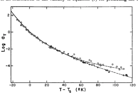
FIG. 8. A plot, taken from ref. 326, of log ay vs. T-T9 for polystyrene¹⁶⁶ (open circles) and polyisobutylene⁸⁶ fractions. The solid line is calculated by equation (7), employing the T, values of Table V. The dashed lines indicate failure of superposition of experimental points for the two polymers at T-T» > 50°.

TABLE V

REFERENCE TEMPERATURES, ° K . , POLYISOBUTYLENE AND POLYSTYRENE FRACTIONS³²⁶

(From Viscosity Measurements¹⁶⁰· ⁶) Polymer

Polyisobutylene⁸

Polystyrene¹⁶⁶

Mol. Wt.

4170 5380 6610 8500 1675 2085 2600 3041 3590 6650 13300 19300

T_a 238 241 240 240 358f 371 380 383 393 395 404 407

1 0

194 197 200 202 313 326 335 338 348 350 359 362

τ.-τ_σ

44 44 40 38 45 45 45 45 45 45 45 45

* Glass transition temperatures, measured for polystyrenes¹⁶⁶ and calculated for polyisobutylenes from a formula given by Fox and Flory.¹⁶⁰

t The values for polystyrenes were actually taken as T0 + 45 instead of from curve fitting.

served values of log aT for polystyrene and polyisobutylene fractions covering a wide molecular weight range, the solid curve of Fig. 8 was cal- culated ^m from the values of T8 given in Table V. Data for all fractions co- incide reasonably well with the composite curve for T-T8 < 50°. At higher temperatures, however, the dashed curves representing the experimental points for the two polymer types diverge.

The data in Table V show that a decrease in molecular weight diminishes Ta by approximately the same amount that it diminishes Tg [in accordance with equation (9)], thus illustrating the approximate validity of equation (7a) and (8a) for these low molecular weight polymers.

Since equations (7) and (8) contain only one arbitrary parameter as con- trasted to three in equations (5) and (6) and since they have been shown to apply universally, not only to all polymers and polymer solutions for which data are available, but also to low-molecular-weight inorganic and organic glass-forming liquids, it is expected that future developments will be based on these rather than on equation (6). For the present, however, we must conclude (cf. Fig. 8) that while equations (7) and (8) are valid empirical expressions in the region of Tg to Tg + 100°, equations (5) and (6) are likely to be more accurate at higher temperatures. The theoretical significance of these equations and their further development will be dis- cussed in a later section.