RESEARCH ARTICLE
Performance measurement of ESG-themed megatrend investments in global equity markets using pure factor portfolios methodology
Helena Naffa☯, Ma´te´ FainID*☯
Department of Finance, Corvinus University of Budapest, Budapest, Hungary
☯These authors contributed equally to this work.
*mate.fain@uni-corvinus.hu
Abstract
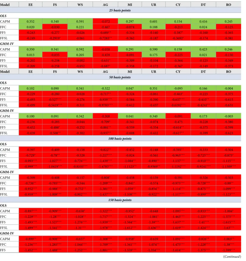
ESG factors are becoming mainstream in portfolio investment strategies, attracting increas- ing fund inflows from investors who are aligning their investment values to Sustainable Development Goals (SDG) declared by the United Nations Principles for Responsible Investments. Do investors sacrifice return for pursuing ESG-aligned megatrend goals? The study analyses the risk-adjusted financial performance of ESG-themed megatrend invest- ment strategies in global equity markets. The analysis covers nine themes for the period 2015–2019: environmental megatrends covering energy efficiency, food security, and water scarcity; social megatrends covering ageing, millennials, and urbanisation; governance megatrends covered by cybersecurity, disruptive technologies, and robotics. We construct megatrend factor portfolios based on signalling theory and formulate a novel measure for stock megatrend exposure (MTE), based on the relative fund flows into the corresponding thematic ETFs. We apply pure factor portfolios methodology based on constrained WLS cross-sectional regressions to calculate Fama-French factor returns. Time-series regres- sion rests on the generalised method of moments estimator (GMM) that uses robust dis- tance instruments. Our findings show that each environmental megatrend, as well as the disruptive technologies megatrend, yielded positive and significant alphas relative to the passive strategy, although this outperformance becomes statistically insignificant in the Fama-French 5-factor model context. The important result is that most of the megatrend fac- tor portfolios yielded significant non-negative alphas; which supports our assumption that megatrend investing strategy promotes SDGs while not sacrificing returns, even when accounting for transaction costs up to 50bps/annum. Higher transaction costs, as is the case for some of these ETFs with expense ratios reaching 80-100bps, may be an indication of two things: ESG-themed megatrend investors were willing to sacrifice ca. 30-50bps of annual return to remain aligned with sustainability targets, or that expense ratio may well decline in the future.
a1111111111 a1111111111 a1111111111 a1111111111 a1111111111
OPEN ACCESS
Citation: Naffa H, Fain M (2020) Performance measurement of ESG-themed megatrend investments in global equity markets using pure factor portfolios methodology. PLoS ONE 15(12):
e0244225.https://doi.org/10.1371/journal.
pone.0244225
Editor: J E. Trinidad Segovia, University of Almeria, SPAIN
Received: May 30, 2020 Accepted: December 7, 2020 Published: December 22, 2020
Copyright:©2020 Naffa, Fain. This is an open access article distributed under the terms of the Creative Commons Attribution License, which permits unrestricted use, distribution, and reproduction in any medium, provided the original author and source are credited.
Data Availability Statement: All relevant data are within the manuscript and itsSupporting Informationfiles.
Funding: The work of HN and MF was supported by the Higher Education Institutional Excellence Program of the Ministry for Human Capacities in the framework of the ‘Financial and Public Services’
research project (NKFIH-1163-10/2019) at Corvinus University of Budapest. The funders had no role in study design, data collection and
1. Introduction
Sustainable investing has become an attractive strategy both for investors and policymakers all around the world. According to theGlobal Sustainable Investment Alliance’s 2018report, sus- tainable investing reached $30.7 trillion at the start of 2018, a 34 per cent increase in two years.
Also, the proportion of sustainable investments relative to total managed assets made up 33 per cent in 2018 while it was 21 per cent in 2012, which corresponds to an almost 60 per cent increase in six years [1]. Nevertheless, due to the lack of consistent definitions, it is difficult to determine the actual size of sustainable finance worldwide; for instance,J.P.Morganestimates
‘only’ $3 trillion [2].United Nations’2030 Agenda for Sustainable Development sets out 17 Sustainable Development Goals (SDGs) and 169 targets which are to balance the economic, social and environmental dimensions of sustainable development [3–5]. Some of the goals are as follows: end hunger, achieve food security (SDG2), ensure healthy lives and promote well- being for all at all ages (SDG3), make cities and human settlements inclusive, safe, resilient and sustainable (SDG11).
Sustainable investing has at least 50 years of history, as the first related publications ofMos- kowitz,Bragdon and Marlin,Bowman and Haire,Belkaoui[6–9] appeared in the ‘70s. How- ever, the concept of sustainable investing covers numerous different strategies and approaches;
besides, several alternative names and terms exist as well. This heterogeneity in both terminol- ogy and investment strategies are apt to give rise to misunderstandings among academics and practitioners [10,11]. For simplicity, we use the widely accepted terms of responsible investing (RI), sustainable investing (SI), socially responsible investing (SRI), environmental-social-gov- ernance (ESG) investing interchangeably throughout the study.
Further, according toGSIA[12], there are seven representative ESG investing strategies:
exclusionary screening, best-in-class screening, norm-based screening, ESG integration, sus- tainability-themed investing, impact/community investing, and corporate engagement. Sus- tainability-themed ESG investment strategies are in the focus of our paper. Based on
UNCTADdefinition [13], ESG-themed portfolios include stocks that only concentrate on one particular sustainability theme (for example, gender equality or low carbon). However, stocks also belong to this group if they primarily focus on only one ESG pillar (environment, social or governance); alternatively, they track a ‘quasi sector’, such as energy efficiency or food security.
We also introduce the term ‘megatrend’ as a closely related concept.NaisbittandBoesl-Bode define megatrends as large transformative social, environmental, economic, political, and tech- nological changes that could dramatically alter daily life [14,15].
Sustainability themed investing approach is among the youngest ESG strategies, given that at the end of 2012, only $70 billion had been invested in ESG-themed funds. Since then, the strategy has shown impressive growth, with total Assets Under Management (AUM) reaching
$1,018 million by the end of 2018. This figure corresponds to 56.23 per cent CAGR [1].
UNCTAD, referring to Blackrock, predicts that the ESG ETF market will exceed $500 billion by 2030 [13].
We analyse the following nine ESG-themed megatrends in the empirical section: energy efficiency, food security, water scarcity (environmental megatrends); ageing, millennials, urbanisation (social megatrends); cybersecurity, disruptive technologies, robotics (governance megatrends). The stocks in each thematic portfolio come from ESG-themed ETFs. Our stock selection approach relies on signalling theory meaning that the relative amount of money inflows targeting megatrend funds signal the portfolio management industry’s belief in those stocks being the best candidates to represent megatrends.
The research question of our paper is to examine whether megatrend investing is valid; that is, we test if megatrend factor portfolios could generate superior returns, on a risk-adjusted
analysis, decision to publish, or preparation of the manuscript.
Competing interests: The authors have declared that no competing interests exist.
basis. We first compare the returns to the passive strategy (viz., we calculate CAPM alphas and Sharpe ratios relative to the market benchmark), and then measure the alpha applying various Fama-French model specifications (e.g. FF three-factor model, FF five-factor model). Our research question can also be interpreted as a test of the efficient market hypothesis (EMH) [16]. We also attempt to infer whether investing in megatrends may help in achieving some of the United Nations’ Sustainable Development Goals (SDGs) [3]. For the complete list of the SDGs see S1 Appendix inS2 File.
Our investment universe covers global equity markets spanning January 2015 and June 2019, which is a relatively short timeframe; however, the inflows into ESG-themed funds, as men- tioned above, do not have a long history, therefore limiting our reference period. Further, there are studies in the corresponding literature on mutual fund performance that have a similarly shorter timeframe [17–19]. We source weekly trading data from Bloomberg and select the widely tracked MSCI All Country World Index (MSCI ACWI) as a benchmark. Besides ESG factors, we define eleven traditional style factors (beta, value, momentum, size, volatility, liquidity, profit- ability, growth, investment, leverage, and earnings variability) derived from 28 firm characteris- tics; 24 industry group factors (based on MSCI’s global industry classification standards, GICS);
and 48 individual country factors to control for secondary factors. Altogether, we compiled a uniquely organised database, that includes approximately 15 million data points, covering roughly 2,700 individual stocks, for a period spanning 234 weeks, and measuring 106 factors.
A suitable methodology is required to capture the actual performance characteristics of the megatrend portfolios. Secondary factor exposures such as size, value, momentum or any other factors, could have a substantial consequence on the performance, i.e. these disturbing effects should be disentangled. To this end, we construct pure factor portfolios which rest on con- strained WLS (CWLS) cross-sectional regressions. The cross-sectional calculations originate from the classic work ofFama-MacBeth[20,21], and it is also in line with current empirical asset pricing literature [22–27]. Filtering out the effects of secondary factors is consistent with the creation of factor-mimicking long-short dollar-neutral portfolios. Concurrently, we avoid the usage of the ‘cumbersome’ double-sort quintile portfolio selection methodology intro- duced byFama and French[28–30]. Next, we analyse the time series of megatrend portfolios’
returns resulting from CWLS by employing OLS with Newey-West standard errors. We also apply a GMM estimator that relies on a new and innovative set of distance instrumental vari- ables (GMM-IVd) to account for the well-known phenomenon that the FF factors usually incorporate different forms of endogeneity [31–35].
The remainder of the paper is organised as follows. In the second section, we introduce the ESG literature, which is followed by a brief insight into the ‘ESG-themed megatrends’ concept.
Next, we highlight the essential features of pure factor portfolios and the GMM-IV approach.
The megatrend portfolio construction technique is also presented in this section. Subse- quently, we introduce the unique database compiled for the empirical analysis. Finally, we present our empirical findings. The paper ends with a conclusion.
2. Literature review
There are many competing terms and definitions of sustainable investing. According toDau- gaard, in the early times, the term ‘ethical’ was the commonly used expression. ‘Ethical’ was then replaced by ‘socially responsible investing’ (SRI). However, the relevance of ‘social’ had become controversial and was frequently replaced with the term ‘sustainable’ or researchers simply negligeed it; hence only the concept of ‘responsible investing’ (RI) remained [10]. Now- adays, ‘ESG’ is also applied routinely. We do not wish to make distinctions between these terms; therefore, we use them interchangeably throughout the text.
Sustainable investing has a rich literature that dates back to the early 1970s. The pioneering study ofMoskowitzargues that responsible corporate behaviour might manifest in superior financial performance [6]. The influence of Moskowitz’s work is incontestable; as evidenced by the fact that the US Social Investment Forum has awarded the Moskowitz prize named in his honour since 1996, for the best article about the financial impact of socially responsible investing [10,36]. In contrast to Moskowitz,Friedmanclaims that including ESG criteria in managerial decisions generates additional costs which, in turn, results in weaker financial per- formance [37]. These two contradictory views, supplemented by a third one on neutrality, have persisted until today and fundamentally determine research initiatives.
As mentioned, there exist three competing hypotheses in the management literature. The first one accepts the views of Moskowitz and emphasises the positive relationship between ESG and financial performance. Various management theories underpin this concept. Stake- holder theory [38–41] or good management theory [42] argue that the satisfaction of primary stakeholders (e.g. customers, employees, local communities, shareholders, natural environ- ment) is critical in achieving superior financial performance. The second hypothesis argues for a negative relationship; namely, higher ESG performance lowers financial performance. The trade-off hypothesis [37,43–46] declares that higher ESG performance is expensive: resource reallocation to socially responsible activities like charity, community development do not pay off [43], but higher operating costs are incurred due to internalisation of externalities [46]. The third hypothesis is the ‘no effect’ premise, which is often attributed toMcWilliams and Siegel [47,48]. The authors claim that incorporating R&D factors in the analysis of the ESG and financial performance relationship eliminate the positive impact, resulting in neutrality.
Over the past fifty years, a tremendous number of studies have been culminated examining the actual relationship between ESG and financial performance. Further, parallel with primary researches, several summarising literature reviews have also been published [49–53]. Probably the most comprehensive one is written byFriede,Busch and Bassen[54] who combine the findings of about 2,200 individual papers using second-order meta-analysis and concluding that roughly 90 per cent of studies found a nonnegative ESG-financial performance relationship.
Our study aims to measure themarket performanceof ESG-themed investing. Though the ESG versus market performance relation is characterised by the same three hypotheses (neu- tral, positive, negative) as those emphasised in the management literature, some specific facets are worth mentioning. The no-effect hypothesis is closely related to the modern portfolio the- ory (MPT) ofMarkowitz[55] and the efficient market hypothesis (EMH) ofFama[16]. The former argues that there is no return premium for factors that bear only idiosyncratic risk, i.e.
it is assumed that ESG risks can be diversified [56]. The latter maintains that stock prices reflect all available and relevant information; hence it is impossible to achieve superior risk- adjusted returns relative to the market portfolio [57].
Some equilibrium models support the ‘trade-off’ hypothesis [46,58,59]. Each suggests that socially responsible stocks have a lower cost of capital either due to incomplete information [58], investor preferences [59] or the internalisation of externalities [46] which, in turn, results in higher valuation and lower future (expected) return [60,61]. Another critical view, accord- ing toBauer,Koedijk and Otten, is that ESG investments are likely to underperform in the long run because ESG portfolios are by nature subset of the market portfolio, i.e. the degree of diversification is lower [56].
Hamilton et al. andRenneboog et al. claim that investors may do well while doing good;
viz., investors earn positive risk-adjusted returns while contributing to a good cause [52,62].
Outperformance happens if ESG screening procedures generate value-relevant information otherwise not available to investors. ‘Value-relevant information’ indicates that the ‘doing well
while doing good’ hypothesis might hold if markets misprice social responsibility [56,62];
therefore, it is against the EMH [52].
According to GSIA, ESG-themed investments are still in their infancy, but they have excep- tional growth potential, which is also supported by the fact that they achieved and maintained a 56.23 per cent CAGR between 2012 and 2018. Due to its short history, to the best of our knowledge, only a limited number of studies have paid attention to ESG-themed (megatrend) investment strategies.Alvarez and Rodríguez[17] focused on the water sector,Malladi[63]
constructed children-oriented indices,Martí-Ballester[5] analysed the performance of SDG mutual funds dedicated to biotechnology and healthcare sectors, whileMuley et al. [18] evalu- ated thematic based infrastructure mutual fund schemes in India. Renewable energy and cli- mate change themes are probably the most popular among scholars.Ibikunle and Steffen[64]
measured European green mutual fund performance,Reboredo et al. [19] question if investors pay a premium for ‘going green’,Martí-Ballester[65–67] also analysed sustainable energy- related mutual funds. At the same time,Dopierała,Mosionek-Schweda and Ilczuk[68] test whether asset allocation policy affects the performance of climate-themed mutual funds in the Scandinavian markets (Denmark, Norway, and Sweden).
Our research contributes to the existing literature by analysing some less emphasised E-, S-, and especially G-themed investment strategies. Further, we apply a combination of pure factor portfolios construction technique and GMM-IVdapproach, which has not been employed in sustainable investment literature yet.
3. Megatrends
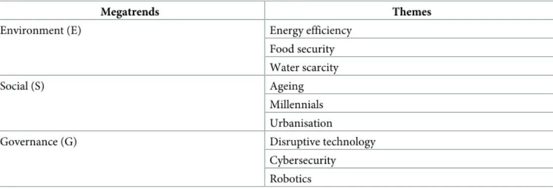
We analyse the following nine ESG-themed megatrend equity portfolios: energy efficiency, food security, water scarcity (environmental megatrends); ageing, millennials, urbanisation (social megatrends); cybersecurity, disruptive technologies, robotics (governance megatrends) (seeTable 1).
Classifying technological megatrends such as cybersecurity, robotics as well as disruptive technologies as governance-related megatrends might not seem to be straightforward. How- ever,Basie von Solms and Rossouw von Solmshighlights that corporate boards are realising that protecting their companies in the cyberspace is, in fact, a corporate governance responsi- bility; consequently, they are accountable for the related cyber risks in their companies [69].
According toFenwick and Vermeulen, disruptive technologies and robotics continue to facili- tate and drive more dispersed forms of corporate organisation–what they call ‘community- driven corporate organisation and governance’ [70, pp. 2–3]. The authors also maintain that technological changes enhance ‘decentralisation and disintermediation’ of business
Table 1. Megatrends and themes.
Megatrends Themes
Environment (E) Energy efficiency
Food security Water scarcity
Social (S) Ageing
Millennials Urbanisation
Governance (G) Disruptive technology
Cybersecurity Robotics https://doi.org/10.1371/journal.pone.0244225.t001
organisations, i.e. these disrupt traditional hierarchical forms. Summing up, the G-themed megatrend portfolios include firms that provide technological solutions related to specific gov- ernance issues. Each megatrend portfolio can be considered as ‘quasi-sectors’ that, at the same time, address ESG concerns.
Besides technological G megatrends, we provide a summary of the investment policies of the E and S themes.Energy efficiencymegatrend invests in companies that provide products and services enabling the evolution of a more sustainable energy sector (for instance, solar and wind energy). Current primary energy demand accounts for 7–9 per cent of GDP and it is expected to grow by at least 1/3 by 2035, hence energy efficiency standards are continuously rising.Food securitymegatrend focuses on companies that operate mainly in agribusinesses:
agricultural equipment, agribusiness and protein, farming, safety inspection firms, health and wellness, waste reduction.Water scarcitymegatrend tracks companies that create products to conserve and purify water for homes, businesses and industries since 750 million people do not have access to clean drinking water.
Ageingmegatrend aims to track the performance of developed and emerging market com- panies exposed to the growing purchasing power of the ageing population. Older persons (60 +) are expected to more than double from 841 million in 2013 to more than 2 billion by 2050.
Typical industry sectors are healthcare, insurance, senior living.Millennialsmegatrend seeks to track the performance of companies that provide exposure to the millennial generation.
Millennials are emerging as a new dominant economic force. They are the largest generation by workforce headcount in the US. Attractive sectors for millennials are accommodation, autos, finance, media, technology, and travel.Urbanisationmegatrend has been designed to replicate, to the extent possible, the performance of energy, industrial, and utility stocks, i.e.
mainly infrastructure companies. The world’s urban population is expected to surpass 6 billion by 2045; therefore, investments that include home-building, infrastructure construction, civil engineering, air/road transport, and utilities could have immense potential.
We rely on signalling theory to select stocks from ESG-themed ETFs and allocate them into thematic megatrend portfolios. According toSpence, signalling theory is about to explain how decision-makers interpret and react in case of incomplete and asymmetrically distributed information among parties to a particular transaction [71]. The theory has its foundation on the premise that one party (e.g. seller) has complete information while external parties (e.g.
buyers), have to rely on what the seller wishes to share.Bergh and Gibbons[72] emphasise that one way for buyers to reduce their risks is to identify observable characteristics that affect the probability of the seller’s performance. Such a characteristic is known as a signal.Spence[73]
defines a signal as activities and characteristics which are visible and convey information in a market. According toConnelly et al. [74], signals are proper to reduce information asymmetry.
Further, they are a form of credible communication that transmits information from sellers to buyers [72].
In our analysis, ETF portfolio managers’ (i.e. sellers) stock selection practices indicate (sig- nal) to investors and analysts (i.e. buyers) that the companies they have carefully chosen are suitable for megatrend investment. Consequently, the relative amount of money inflows into megatrend funds signals the market’s belief in those stocks being the best candidates to repre- sent megatrends. Our signalling theory approach rests on the assumption that market partici- pants (viz., ETF portfolio managers) intend to select stocks that do belong to the various ESG megatrends. Conversely, if the stocks are ‘conventional’ and the ESG megatrend flag is only used as a ‘buzzword’, we may come to a wrong conclusion on the megatrends’ market perfor- mance.Revelli and Viviani[66] also raise this problem, which is the well-known concept of
‘window-dressing’ [75,76]. In the next section, we introduce the formula with which one can calculate a company’s exposure to a particular megatrend.
4. Methodology
AsClarke et al. [23,77] argue, the performance measurement of investment strategies requires two phases. The first one is to implement cross-sectional analyses (not necessarily regressions) to calculate factor returns (for a comprehensive summary of various factor models seeWalter and Berlinger[78]). Secondly, time-series analyses (again, not necessarily regressions, see [25]) are applied to estimate portfolio alphas and sensitivities to the predetermined set of factors. In the literature, theFama-French (FF)[28–30] and theFama-MacBeth (FM)[20,21] procedures are the two most commonly employed approaches to attain factor returns. Our empirical anal- ysis rests on FM; however, in the following paragraphs, we briefly compare the underlying
‘philosophy’ of the two methods, to justify our choice. Next, we introduce the mathematical background of the FM method and the innovative GMM-IVdused for times series analysis.
The section ends with the formula applied to calculate megatrend exposures.
The well-known portfolio sorting technique of FF is the dominant analysis tool in empirical asset pricing [79–84]. Despite several favourable properties such as simplicity or the lack of any required functional format, it also has some drawbacks. One is that extending the number of explanatory factors beyond a certain number makes the modelling cumbersome [23].
Another problematic issue is the quasi arbitrary choice of the number of securities in the top and bottom portfolios (i.e. quintiles, deciles), which results in the exclusion of many stocks;
thus, valuable information is lost [85]. Further, Fama-French rebalances the portfolios under- lying SMB, HML, RMW, CMA only annually (at the end of June), that is, the factors might rely on stale information [26,86]. Finally, in their recent article,Fama and French[25, p. 1893]
summarise the essence of the FF5 factortime-series analysisas follows: it optimises the loadings on factors that are, in fact, not themselves optimised.
The FM method applies regressions that correct most of the FF procedure’s drawbacks but introduces new ones. Firstly, it simultaneously controls for several secondary exposures which is indeed a crucial requirement. Next, it uses the whole investment universe, not just the top and bottom quantiles. Further, it rebalances the factor portfolios at the beginning of each period. The drawbacks are the following: it is parametric (requires a strict functional format), endogeneity problems may emerge (e.g. errors-in-variables, omitted variables), and microcaps as wells as influential observations could have a significant impact [87].
Turning to the method of time series analysis,Fama and Frenchemphasise four approaches of applying the output of cross-sectional analyses (either FF or FM) to explain market anoma- lies [25]. The first one (I.) is the traditional FF modelling technique using time-series (TS) FF factors (i.e. SMB, HML, RMW, CMA) in time-series regressions. The second (II.) is to apply cross-sectional (CS) FM factor returns in time-series regressions. The next approach (III.) is about ‘stacking’ FM (CS) regressions across periods (t); thus it becomes an asset pricing model (model, not regression) that can be used in time-series applications. Finally, the application of an approach that augments the FF TS modelling procedure with interaction variables that allow loadings for SMB, HML, RMW, and CMA to vary with the corresponding firm charac- teristics of FM (IV.).
In the empirical section of this study, we use the second approach (II.) to analyse the risk- adjusted performance of ESG-themed megatrend factor portfolios.Back et al. [26] applied (II.) and found that it explains five market anomalies out of thirteen, while FF (i.e.I.) was not able to clarify any of them.Fama-French[25] evaluate the performance of the four modelling tech- niques and argue that (II.) performs a bit better than (I.). However, the authors contend that (III.) provide a better description of returns than the other ones. Nevertheless, it is worth keep- ing in mind the remark byBack et al. [26, p. 4] that in the absence of an accepted theory
explaining why there are risk premia associated with size, value, profitability, and investment;
there cannot be a universally best method to define factors based on these characteristics.
4.1. Pure factor portfolios
We apply constrained multivariate cross-sectional regression analysis; specifically, we create pure factor portfolios (PFPs). The methodological details presented in this section can be found, inter alia, in [22–24,77,88,89]. Furthermore, cross-sectional regressions are the basis of fundamental equity risk factor models provided by firms such as Axioma, Bloomberg, and MSCI [77]. In our analysis, the applied factors and firm characteristics rest on the factors of the Bloomberg fundamental factor model (see [90]), although we introduce some minor modifications.
Pure factor portfolios have the advantage of removing secondary factor effects without hav- ing a ‘black box’ nature of portfolio construction. Filtering out secondary factor exposures and isolating the effects of ESG factors, as mentioned above, is a crucial methodological require- ment [91].Galema et al. show that the book-to-market factor of the Fama-French model could incorporate some of the ESG characteristics [61]. In the 1980s,Grossman and Sharpealso found that the positive market-relative performance of the South Africa-free portfolios can be attributed to small firm size effect [92].
In the upcoming paragraphs, we first outline the original FM procedure briefly, then the mathematical background of our extended FM approach. Finally, we compare the two meth- ods. The following mathematical derivation of the FM method and supplemental explanations can be found, among others, inFama[21, Chapter 9, pp. 326–329],Fama-French[25], Cochrane[93], andBack et al. [26,27]. The FM estimator is calculated by running cross-sec- tional regressions at each moment in time. With matrix algebra notation:
Rtþ1¼Zt^Ftþ1þutþ1; ð1Þ
whereRt+1is the (N x 1) vector of stock returns onNindividual securities fromttot+1;Ztis the (N x K) matrix of standardised firm characteristics at datet(z-scores), with a vector of ones as its first column;F^tþ1is the (K x 1) vector of the ordinary least squares (OLS) values of the regression coefficients att+1, andut+1is the (N x 1) vector of security return disturbances fort+1(Kis the number of explanatory variables, including the market).
The OLS values for the regression coefficients are as follows:
F^tþ1 ¼ ðZ0tZtÞ 1Z0tRtþ1 ð2Þ
Note that the individual security weights in each factor portfolio are the elements of matrix Wt:
Wt≝ðZ0tZtÞ 1Z0t ð3Þ
One must emphasise that the portfolio weights are observable att, even though the returns, hence the slope coefficients (F) are not observable untilt + 1.
To determine the properties of the slope coefficients, we study the properties ofZt. Note first that
WtZt¼ ðZ0tZtÞ 1Z0tZt¼It; ð4Þ whereItis the (K x K) identity matrix. Given (4) and the fact that the first column ofZtis an (N x 1) vector of 1’s, the FM procedure has some notable features [25, p. 1892]. Firstly, theF coefficients for each variable in an FM cross-section regression is thet+1return on a portfolio
of the left-hand-side assets with weights for the assets that set the monthtportfolio exposure of that given variable to one and zero to other explanatory variables. Secondly, each FM slope portfolio requires zero net investment; that is, the short positions of the left-hand-side assets finance the long positions in other left-hand-side assets. Finally, the intercept is the montht+1 return on a standard portfolio of the left-hand-side (LHS) assets with security weights that sum to one and zero out each explanatory variable. The intercept, which is the level return, is the montht+1return common to all assets and not captured by the regression explanatory variables.
From a mathematical-statistical perspective,ourpure factor portfolios (viz., FM procedure) rest on constrained weighted least squares (CWLS) multivariate cross-sectional regressions, which we explain in more details below. It is worth mentioning, however, that there is also a practical reason to construct PFPs: the method is available now on Bloomberg terminals for portfolio managers around the world, who can apply it in their daily decision-making pro- cesses (see Factors to Watch (FTW) function, Pure factor returns tab in Bloomberg). Neverthe- less, the function is limited to developed markets at the time of writing.
This paper aims to compare the performance of pure megatrend factor portfolios with the benchmark market index and other traditional FF factors to find out whether megatrend fac- tors could outperform it. To this end, market returns, and pure factor portfolio returns are cal- culated. PFP return calculation rests on the following formula:
prtþ1 ¼PN
i¼1pwnt�rntþ1; ð5Þ
whereprt+1is the return of the given PFP att+1,pwntis the pure factor weight of securitynat datet, andrnt+1is the return of securitynatt+1.
The construction of PFPs uses traditional investment styles such as value, momentum, size or industries and countries measured by dummy variables. Calculation of stock weights rests on multi-factor constrained WLS regressions. By calculating the weights, the given factor port- folio will have a unit exposure relative to the benchmark. Parallel, it has market-neutral expo- sures to all other styles, including industries and countries. Industry and country neutrality means that the pure style portfolio has the same industry and country structure as the bench- mark. PFPs are ‘fully invested’ long-short factor mimicking portfolios. To sum up, the critical issue is to measure pure stock weights,pwnt.
The starting point is to write the cross-sectional regression equation on stock returns (for convenience, we drop the ‘hat’ operator from now on):
rntþ1 ¼rMtþ1þP
sznstfstþ1þP
ixnitfitþ1þP
sxnctfctþ1þuntþ1; ð6Þ
wherernt+1is the return of stocknatt+1,rMt+1is the return of the market factor att+1,znstis the standardised exposure of stocknto style factorsat timet,fst+1is the active (market-rela- tive) return of the style factor at timet. Similarly,xnitandxnctare the exposures of stocknto industryiand countrycatt;fit+1andfct+1are active returns for industryiand countrycat timet. Theunt+1is unexplained by the factors and is termed idiosyncratic, or stock-specific.
The stock-specific returns are assumed to be mutually uncorrelated, and uncorrelated with the model factors.
From (6) it is apparent that every stock has unit exposure to the market factor (i.e., this average return is ‘modified’ by thefactive returns). By contrast, dummy variables represent the country and industry exposures: a stock has unit exposure to its industry and country, and zero exposures to all the others. Style factor exposures are standardised scores (z-scores), which have a capitalisation-weighted mean of zero and standard deviation of one (i.e. stocks with negative exposure score below the average of the market).
Weighted standardisation (see [23,77]) should be used for the rescaling process of raw or prior style exposures (e.g. P/E ratios for the value factor). This procedure ensures the consis- tency between the weighting scheme of the benchmark and the weights used to rescale prior style factor exposures. Since our benchmark is the MSCI ACWI Index which is a cap-weighted index, we apply the market capitalisation-weighting scheme. The formula is as follows:
zns¼ xns PN
n¼1wnM�xns
ffiffiffiffiffiffiffiffiffiffiffiffiffiffiffiffiffiffiffiffiffiffiffiffiffiffiffiffiffiffiffiffiffiffiffiffiffiffiffiffiffiffiffiffiffiffiffiffiffiffiffiffiffiffiffiffiffiffiffiffiffiffiffiffiffiffiffiffi
PN
n¼1wnM�x2ns ðPN
n¼1wnM�xnsÞ2
q ; ð7Þ
wherexnsis the prior exposure of securitynto a particular style factors,wnMis the market weight of securityn. In the numerator, we subtract the capitalisation-weighted average of the prior exposure of stylesfrom the prior style exposurexns, and then the difference is divided by the standard deviation of the prior exposure.
After introducing our cap-weighted standardisation convention, we return to (6), but now we use the more convenient matrix notation (note that (8) is the same as (1)):
Rtþ1¼ZtFtþ1þutþ1; ð8Þ
whereRt+1is the (N x 1)vector of stock returns at timet+1,Ztis the (N x K)standardised fac- tor exposure matrix (using (7)),Ft+1is the (K x 1)vector of active factor returns, andut+1is the (N x1) vector of unexplained residuals (the first element of vectorFis the market return, which is, by definition, not an active return).Kequals the total number of factors, including the market factor; hence, the first column ofZtcontains 1’s (exposures to the market factor).
We label the exposure matrix with ‘Z’, although not all the values are standardised: market, industry and country factor exposures are 1 and (0, 1), respectively.
One must recognise two exact collinearities in our model as the sum of industry and coun- try factor exposures give one each (i.e. identical to the market factor). In other words, onlyK-2 variables are genuinely independent; therefore, we must impose two constraints to obtain the Zmatrix have linearly independent columns (without constraints the regression cannot be solved as(Z’Z)-1does not exist, i.e. it is singular). The sum of industry and country returns equals the market return; hence, the market-relative industry and country returns should equal zero.Heston-Rouwenhorst[94],Menchero[22] applied these equations to eliminate exact multicollinearity. The simple mathematical formulae are as follows (witandwctare the market capitalisations for eachiindustry andccountry factor at timet):
P
iwitfitþ1 ¼0 ð9Þ
P
cwctfctþ1¼0 ð10Þ
We can write the constraints in matrix form:
Ftþ1¼CtGtþ1; ð11Þ
whereCtis theK x (K—2)constraint matrix at datet, andGt+1is the(K—2) x 1vector of auxil- iary returns in timet+1. Below, (12) is an example forCtGt+1. Here, for the sake of simplicity, four factors, including the market and three industry factors are involved; therefore, only one
constraint applied:
rM fi1 fi2 fi3 2 66 66 64
3 77 77 75
¼
1 0 0
0 1 0
0 0 1
0 wi1=wi3 wi2=wi3 2
66 66 64
3 77 77 75
gM gi1 gi2 2 66 4
3 77
5; ð12Þ
The heteroscedastic nature of the stock-specific returns (ut+1) and the influence of small stocks is well-known; therefore, weighted least squares (WLS) regressions ought to be applied.
There are more technical opportunities to manage these challenges; therefore, we follow the work ofClarke et al. [77] when we use market capitalisation as weights. The authors argue that it is quite common to use equal weights and square-root-of-market-capitalisation-weights (many commercial risk-factor models use this), the latter, however, produces similar results to the market capitalisation weighting scheme.
We use the (N x N)Vtdiagonal matrix in (13) and substituteCtGt+1(11) forFt+1. The diago- nal elements ofVtare the securities’ market capitalisations (wnM) att:
VtRtþ1 ¼VtZtCtGtþ1þVtutþ1; ð13Þ
Some changes in the variables make (13) a bit simpler (R~tþ1= VtRt+1,Yt= VtZtCtandu~tþ1= Vtut+1):
R~tþ1¼YtGtþ1þ~utþ1: ð14Þ
Now, in (14), we have the standard homoscedastic regression equation again. The OLS solution is as follows:
Gtþ1¼ ðYt0YtÞ 1Yt0R~tþ1: ð15Þ
Making substitutions to transform back the variables, we obtain the final solution:
Ftþ1¼CtðCt0Zt0VtZtCtÞ 1Ct0Zt0VtRtþ1: ð16Þ In (17), we denote the(K x N)matrix of pure factor active weights of securities withPWt
(active weights mean, similarly to active returns, the weight of securities above or below the market weights, i.e. the over- or underweighting relative to the market):
PWt≝CtðC0tZt0VtZtCtÞ 1Ct0Zt0Vt: ð17Þ According to (17), the active security weights in PFPs can be calculated directly by using the cap-weighted standardisation procedure for firm characteristics based on (7). The product of pure security active weights, and the realised stock returns is the return of the pure factor portfolio in (5). The calculation of PFP returns can be derived alternatively, by using the slope coefficients (i.e. market return and factor portfolio active returns) in the CWLS cross-sectional regression of stock returns,Rt+1, on standardised factor exposures,Zt, in Eqs (8) or, equiva- lently, in (16).
At last, we compare the weight matrices of the original (Wtin (3)) and the modified FM procedure (PWtin (17)) to give a summary about the differences. The adapted CWLS regres- sion has the following enhancement compared to the classicalFama-MacBethregression tech- nique (the explanations below, regarding the improvements, could be found in the studies of Clarke et al. [77, p. 16, and online appendix A] andMenchero[22]).
If one looks at the formulae, the first impression may be that (17) is more intricate; that is, it indeed considers issues that (3) does not. Firstly, the observations in each cross-sectional regression are weighted by market capitalisation, viz., we use theVtdiagonal matrix, which is missing in (3). Thus, including smaller stocks has little impact on the regression results, except that more missing or outlier values emerge among the explanatory variables. Secondly, each of the style and megatrend characteristics is shifted every period to have a cross-sectional capitali- sation-weighted mean of zero. Together with observation weighting, this step makes the esti- mated regression intercept precisely equal to the return on a capitalisation-weighted portfolio of all admitted stocks. Non-zero values for the other four factors then measure exposures that are relative to the market portfolio. Further, every descriptor is scaled each period to have a cross-sectional standard deviation of one. In summary, (17) applies the “mean” and the “scale”
adjustments for the firm characteristics based on capitalisation weighted standardisation of (7) while (3) uses arithmetic (i.e., equal-weighted) means and standard deviations for standardisa- tion. Finally, we use constraints (Ct) to manage exact multicollinearities, consequently, be capable of filtering out secondary industry and country exposures, which is not the case for the original FM method.
4.2. Time series analysis with GMM-IVd
After calculating PFP returns, the next step is measuring and testing the megatrend portfolios’
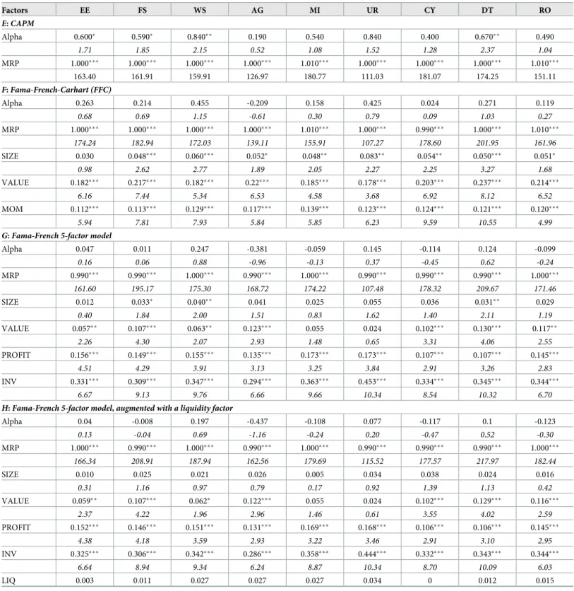
alphas using time-series regressions. In the empirical section, we test the traditional CAPM, the Fama-French-Carhart (FFC), the Fama-French 5 factor (FF5) and the augmented version of the FF5 factor model that includes liquidity as a sixth factor (FF5L). Eq (18) is the CAPM:
RPet¼aeþb1eMRPtþuet; ð18Þ whereRPetis the excess return (Ret—Rft) of megatrendeatt(we useeas the abbreviation for ESG-themed megatrend);Rftis the one-year US Treasury bill rate;αeis the Jensen’s alpha;
MRPtis the market risk premium (RMt−Rft) att;b1eis the beta of megatrende(sensitivity to the market), anduetis the error term. CAPM is an appropriate model for testing the perfor- mance of ESG-themed investments relative to the passive strategy.
Eq (19) is the FFC four-factor model:
RPet ¼aeþb1eMRPtþb2eFSIZEtþb3eFVALUEtþb4eFMOMtþuet; ð19Þ whereFSIZEt,FVALUEt,FMOMtare, respectively, the market-relative pure factor returns from (16) for size, value, and momentum firm characteristics. The regression coefficientsb2e,b3e, b4eare the ESG-themed portfolios’ sensitivities to the prespecified factors. We employ the FFC model to account for the effects of momentum.
The next model is the FF5 factors:
RPet¼aeþb1eMRPtþb2eFSIZEtþb3eFVALUEtþb4eFPROITtþb5eFINVtþuet; ð20Þ whereFPROFITt,FINVtare PFP returns for profitability and investment factors. The coefficients b4eandb5eare the left-hand-side assets’ sensitivities to profitability and investment factors.
The last model is the FF5 augmented with a liquidity factor:
RPet¼aeþb1eMRPtþb2eFSIZEtþb3eFVALUEtþb4eFPROITtþb5eFINVtþb6eFLIQtþuet; ð21Þ In the empirical asset pricing literature, it is a common practice to identify new factors besides the traditional Fama-French exposures (Cochrane[95], thus, not inadvertently used the term ‘zoo of factors’). The effect of liquidity or illiquidity is a critical factor which is clearly in the focus of researchers (seeAmihud[96],Pástor and Stambaugh[97] orRacicot et al. [98,
99]). Beyond liquidity, the applied factors are, in fact, very diverse:López-García et al. [100]
applied a long term memory factor,Chan et al. [101] used R&D and advertising expenses, Thomas and Zhang[102] analysed the performance of inventory changes.
The critical methodological question is how to estimate the coefficients of each equation.
We applied two methods: 1.) traditional OLS withNewey-West(HAC) standard errors [103], and 2.) generalised method of moments using innovative, robust distance instrumental vari- ables (GMM-IVd), which can be found inRacicot[31],Racicot et al. [32,104] andRoy-Schijin [35]. The GMM-IVdmethod is suitable to address the various manifestations of endogeneity inherent in factor models [105]. According toRacicot[31], the GMM-IVdapproach provides solutions to measurement errors (errors-in-variables), specification errors.
FollowingRacicot and Rentz[104] the GMM estimator in (22) chooses the value,^be, that minimises a quadratic function of the moment conditions. We define the estimator as follow (we changed the notation ofRacicot and Rentzslightly to have consistent formulae with the previous equations):
^be�argmin^b efT 1½d0ðRP F^beÞ�0WT 1½d0ðRP F^beÞ�g ð22Þ
The GMM-IVdestimator makes the moment conditions as close to zero as possible. Each variable in (22) is defined below in (23) to (34). We start withT, which is the total number of observations (i.e. periodst = 1,. . .,T).Wis a symmetric positive-definite matrix known as a weight matrix with the same number of rows and columns as the number of columns ofd. We estimate W with the Newey-West HAC estimator. RP is defined as follow:
RP¼F^beþu ð23Þ
whereFis assumed to be an unobserved matrix of explanatory variables. The observed matrix of observed variables is assumed to be measured with normally distributed error:
F�¼Fþv ð24Þ
^beis defined as:
^be¼^be2SLS¼ ðF0PZFÞ 1F0PZRE ð25Þ
Pzis defined as the standard ‘predicted value maker’ or ‘projection matrix’ used to com- pute:
PZ ¼ZðZ0ZÞ 1Z0; ð26Þ
In (26),Zis the matrix of instruments (should not be confused withZfrom section 4.1.).
Here, Z is obtained by optimally combining theDurbin[106] andPal[107] estimators using GLS.
Using the projection matrix, we can calculate the predicted values ofF:
PZF¼ZðZ0ZÞ 1Z0F¼Z^y¼F^ ð27Þ
From (27) extract the matrix of residuals
d¼F ^F¼F PZF¼ ðI PZÞF ð28Þ
In (28)dis a matrix of instruments that can be definedindividuallyin deviation form as
dit¼fit ^fit ð29Þ
AsRacicot[31, p. 986] highlights (29) may be considered as a filtered version of the endoge- nous variables. It removes some of the nonlinearities embedded in thefit. Formula (29) is thus a smoothed version offitwhich might be regarded as a proxy for its long-term expected value, the relevant variables in the asset pricing models being theoretically defined on the explanatory variables’ expected values.
The next step is to calculate the values of^fitwhich is obtained by performing OLS regres- sions based on thez(cumulant) instruments:
fit ¼^g0þz^φþBt¼^fitþBt ð30Þ
(30) amounts to running a polynomial adjustment on each explanatory variable.
The z isntruments are defined as z = {z0,z1,z2}, where
z0¼iT ð31Þ
z1¼fJ
f ð32Þ
z2 ¼fJ fJ
f 3f½ðDðf0f=TÞ� ð33Þ
Dðf0f=TÞ ¼plim
T!1ðf0f=TÞJ
Ik ð34Þ
In (31)ιTstands for a vector of one (T x 1). In (32)–(34)fis the matrix of the explanatory variables expressed in deviation from their mean; the operator⊙is the Hadamard product;D (f’f/T)is a diagonal matrix andIkis an identity matrix wherekis the number of explanatory variables. Again, z1contains the instruments used in theDurbin[106] estimator, and z2con- tains the cumulant instruments employed byPal[107]. Racicot and Rentz [103, p. 332]
emphasise that the assumption of normality is a sufficient condition for the estimators to be consistent once measurement errors are purged using these third and fourth cross-sample moments as instruments for parameter estimation.
4.3. Calculating megatrend factor exposures
To quantifymegatrend exposures, using dummy variables would seem an obvious solution:
one could collect exchange-traded funds (ETFs) that consider themselves as thematic invest- ment funds, then each company in these ETFs are classified into a particular megatrend, hence get a value of one. Those firms that are not listed in any of the thematic ETFs get a value of zero. In contrast, our idea is that megatrend exposures ought to be measured on a ratio scale as companies are different regarding how much they are affected by different megatrends, viz., how well they fit into megatrends. (Further, applying dummy variables would introduce another exact multicollinearity in our model, which is, in fact, not a real challenge to handle, but makes the modelling a bit more complicated.) The applied formula for megatrend expo- sures is, therefore, as follows:
MTEnmt¼
PE
e¼1FInmt
MCapnt ; ð35Þ
whereMTEnmtis the megatrend exposure of stocknin megatrendmat timet.FInmtis the total
fund inflow (the total number of sharenmultiplied by its stock price) into ETFethat invests in stocknand belongs to a particular megatrendmat timet(there are a total ofEETFs), and MCapntis the total market capitalisation of stocknat timet. The higher the ratio, the higher the exposure of a given stock to a particular megatrendm.
To haveFIs, we analysed 37 ETFs that consider themselves as thematic funds (see them in S5 Appendix inS2 File). All the ETFs had more than $40 million AUM at the end of September 2019 (27.09.2019). The total AUM was $16,943 million. We should emphasise that, due to data limitations, we use constant positions (the number of stocks remains unchanged during the entire period, and reflects the status as of 20.09.2019.). Nevertheless, the stock prices vary weekly to quantify fund inflows for each week between 2015 and 2019.
5. Dataset
To obtain valid results, the sound choice of the investment universe is essential. According to Cahan and Ji, there are two types of security universes: coverage universe and estimation uni- verse [90]. We employ a global investor perspective throughout this paper, that is, coverage universe includes theoretically ‘all’ the stocks that are traded in global markets. However, for practical reasons, a widely used index is satisfactory. We use the MSCI All Country World Index, which had more than 2.700 constituents in 2018. The estimation universe is the subset of stocks from the coverage universe used for constructing pure factor portfolios. The availabil- ity of critical variables such as stock price, total return and market capitalisation apart from standard data cleansing procedures determines the size of the estimation universe.
We collected weekly stock data from Bloomberg covering January 2015 and June 2019 on MSCI ACWI Index members to calculate total returns, nine megatrend exposures, 28 prior style descriptor exposures, 24 industry (based on second level GICS) and 48 country dummies.
Prior styledescriptorsare the inputs to compute stylefactorexposures with principal compo- nent analysis (PCA). As a result of PCA, we get eleven style factors (seeTable 2). (S2 Appendix inS2 Filecontains the detailed descriptions, calculation methods and applied Bloomberg codes related to each factor.)
All the stocks that were traded between 2015 and 2019 are analysed, which helps to elimi- nate survivorship bias. For precise statistical inference, we performed data cleansing proce- dures on a year-by-year basis. First, we excluded those companies that did not have, for any reasons, market price, total return or market capitalisation data. Second, the so-called penny stocks (stocks with a maximum price below five dollars) were removed (in line with [26,87]).
Unfortunately, despite our best efforts, we had missing values for several descriptors and for many firms, which is not surprising as 28 company characteristics are analysed. S3 Appen- dix inS2 Filepresents the proportion of missing observations for each characteristic: one can see that 1.81 per cent of observations is missing which is relatively moderate (CF/P has the highest missing rate with 12.01 per cent); however, this represents 200–300 companies (i.e.
many firms have only a few missing values). One solution could have been to delete these observations listwise; however, that would have decreased our sample size radically. Instead, we implemented multiple imputation (MI, [108]) procedures (we used Stata16). Due to the rel- atively low proportion of missing data, only three imputations were executed. We employed the Markov Chain Monte Carlo (MCMC) imputation procedure, and all the 28 descriptors were used.
The MCMC procedure assumes that all the variables in the imputation model have a joint multivariate normal distribution (MVN), probably the most common parametric approach for MI [109]. The specific algorithm used is called the data augmentation (DA) algorithm, which is an iterative MCMC procedure. The algorithm fills in missing data by drawing from a
conditional distribution, in this case, an MVN, of the missing data given the observed data (for a detailed explanation of DA in Stata environment see [110]). In most cases, simulation studies have concluded that the assumption of MVN leads to reliable estimates even if the normality assumption is violated given sufficient sample size [111,112].Table 3summarises the sample sizes year by year; hence the MCMC is an appropriate procedure for our analysis.
Next, we specified winsorisation limits to ensure that extreme values would not affect statis- tical inferences (in line with [87]). The limits were the 1stand the 99thpercentiles of each descriptor. We replaced each extreme descriptor value with the 1stand the 99thpercentile.
The estimation universe covers on average 75 per cent of the benchmark, which we con- sider as sufficient. Due to consistency considerations, we construct a market-cap weighted
Table 2. Pure style factors and factor-related descriptors.
Factor Descriptor
Beta (B) Market-relative beta:Beta-1
Value (V) E/P
CF/P BV/P
Momentum (M) Return momentum
Price momentum Sharpe-momentum
Size (S) • ln(MCap)
• ln(Assets)
• ln(Sales)
Volatility (Vol) Total volatility
Residual volatility Price range
Liquidity (L) Amihudliquidity ratio
Profitability (P) ROE
ROA ROIC/WACC Profit margin
Growth (G) EBT growth
Net income growth Sales growth
Investment (I) Asset growth
Leverage (L) Book leverage
Market leverage Debts/Assets
Earnings variability (EV) Sales variability
Net income variability FCFF variability Source: Own compilation based on Bloomberg’s US fundamental factor model [90].
https://doi.org/10.1371/journal.pone.0244225.t002
Table 3. Sample size after data cleansing and multiple imputation procedures.
Sample size 2015 2016 2017 2018 2019
MSCI ACWI members (30th June) 2 483 2 481 2 500 2 781 2 849
Companies in the final sample 1 915 1 893 1 953 2 031 2 040
Sample size/MSCI ACWI members 77.12% 76.30% 78.12% 73.03% 71.60%
https://doi.org/10.1371/journal.pone.0244225.t003
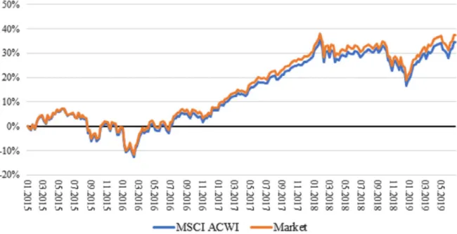
portfolio (Market) of the estimation universe, which serves as the reference point in cross-sec- tional regressions. InFig 1, one could see the cumulative total log-returns of MSCI ACWI and our ‘artificial’ Market portfolio. The prices move together and almost overlap each other (the cumulative return difference is 2.88 per cent for the entire period). It is good news since the created Market portfolio is the reference point to calculate active weights (and returns) of pure factor portfolios. The performance measurement of pure megatrend factor portfolios is mea- sured relative to the benchmark index (MSCI ACWI).
After prior style descriptor calculations and data cleansing, as well as multiple imputation procedures, we use principal component analysis (PCA) for every week to calculate descriptor weights. The PCA results in the dimension reduction of descriptors. As a result of the PCA, we obtain eleven traditional style factors: market-relative beta, value, momentum, size, volatility, liquidity, profitability, growth, investment, leverage, and earnings variability.
The concept of market-relative beta hinges on the modified CAPM equation, and it is as fol- lows:
Rn¼RMþ ðbn 1ÞRM; ð36Þ
whereRnandRMare the excess returns for stocknand the market, and (βn—1) is the market- relative beta. According to the traditional CAPM, the expected return on unscaled relative betas (i.e. before standardisation) should be equal to the market risk premium, which is the slope coefficient of the security market line (SML). When active returns are calculated (i.e.
after standardisation) the return premium should be zero if CAPM assumptions hold. If the return premium is negative, the slope of SML is flatter or even downward sloping. Empirical researches [113] found that the SML is, in most of the time, flat or downward sloping (hence the name ‘low beta anomaly’). An alternative way of thinking about risk is inOrmos-Zibriczky [114]. The authors investigated entropy as a financial risk measure. Entropy explains the equity premium of securities with higher explanatory power than the classical beta parameter of the CAPM.
Fig 1. Cumulative total log return of MSCI ACWI Index and market portfolio. The market portfolio contains only companies that have prices, total returns and market capitalisations, and are not considered as penny stocks. “Market” portfolio is the reference point for the cross-sectional regressions. MSCI ACWI is the benchmark for the time series analysis.
https://doi.org/10.1371/journal.pone.0244225.g001