Performance Measurement of Active Investment Strategies Using Pure Factor Portfolios*
Máté Fain – Helena Naffa
The article uses pure factor portfolios formed by multivariate cross-sectional regressions to examine whether these active investment strategies could achieve excess return relative to passive strategies. The hypothesis can also be construed as a test of market efficiency. The study includes ten style factors. Our empirical study shows that a consensus buy strategy of the pure value factor yielded significant positive excess returns in the past almost 20 years. Size and momentum factors characterised in the literature by positive excess return are not significant in our study. Excess return of the factors capturing riskiness (earnings variability, volatility, leverage) is significant and negative, which corroborates with our expectations, rendering a consensus sell investment strategy successful, based on these factors.
The profitability, growth and trading activity factors produced results contrary to our expectations; therefore, excess return could have been achieved via a contrarian selling strategy. Our research results are consistent with the weak form of market efficiency analyses.
Journal of Economic Literature (JEL) codes: G11, G12, G14, G15.
Keywords: equity markets, asset pricing, return, pure factor portfolio, multivariate regression, performance measurement, market efficiency
1. Introduction
The active professionals engaged with financial investments and scientific researchers have always been intrigued by the question how to forecast and interpret the fair expected return of securities reflecting risk1 and ultimately equity prices.2 The various capital market theories and applications devised in past decades
* The papers in this issue contain the views of the authors which are not necessarily the same as the official views of the Magyar Nemzeti Bank.
Máté Fain is a PhD Student at the Corvinus University of Budapest. Email: mate.fain@uni-corvinus.hu Helena Naffa is a Senior Lecturer at the Corvinus University of Budapest. Email: helena.naffa@uni-corvinus.hu The Hungarian manuscript was received on 17 December 2018.
DOI: http://doi.org/10.33893/FER.18.2.5286
1 There is a major difference between expected return and the required rate of return, which should be borne in mind. See, for example, Fernandez (2015) and Fernandez – Acín (2015).
2 More precisely, investors are interested in total return, comprising the sum of dividend yield and price changes. In this study, return always means total return.
focused on identifying the various factors influencing returns and on establishing a significant link between expected return and risk.
How has financial and investment thinking changed over the last roughly 50 years?
The analytical framework of stocks’ intrinsic value emerged in the 1930s. The major methodological tomes are attributable to Williams3 and Graham – Dodd4 (Malkiel 2001). Modern finance was born and consolidated in the 1950s and 1960s. This period was characterised by economists and their theories such as the modern portfolio theory of Markowitz (1952) or the capital asset pricing model (CAPM) of Sharpe (1964), Lintner (1965) and Mossin (1966). Contemporary thinking featured rational investors, efficient markets from an information perspective (see Fama 1970) and approaches that interpreted the development of returns as random walk.
Around the 1970s, the belief that markets are probably not “that” efficient as previously supposed, and that investors do not always behave rationally slowly became accepted in financial thinking.5 The assumptions and conclusions of the CAPM were increasingly questioned; in response, multifactor models started to dominate (see the Arbitrage Pricing Theory by Ross 1976). The literature usually attributes the spread and popularisation of the multifactor models to Fama – French. By now, researchers in the field have identified roughly one hundred factors that could explain returns. In any case, it is not easy to decide which of these can be deemed significant in this universe of factors, both statistically and from the perspective of practical interpretability. Cochrane (2011) aptly referred to this multitude as a factor zoo.
Our study uses pure factor portfolios formed by multivariate cross-sectional regressions to examine whether these active investment strategies could achieve excess return relative to passive strategies. The hypothesis of the paper can also be regarded as a test of market efficiency. The universe of the analysis comprises the equity market of the United States between 2000 and 2018, while the benchmark is the Russell 3000 Index. The indicators used for assessing the performance of the factors are Jensen’s alpha and the Sharpe ratio.
The sections below first describe the major studies criticising the capital asset pricing model and the efficient market theory and also present the market pricing anomalies (Section 2). After the anomalies, the focus shifts to various multifactor models explaining returns, mainly the works of Fama and French (Section 3). After reviewing the literature, studies are presented that used pure factor portfolios to
3 The Theory of Investment Value
4 Security Analysis
5 This is the period of the emergence of behavioural finance, the foundations of which were laid down by Kahneman and Tversky with their seminal work published in 1979 (Prospect Theory).
analyse various returns (Sections 4 and 5). Before turning towards the empirical part of the paper (Section 7) the database used is described in detail (Section 6).
Section 8 summarises the main messages of the paper.
2. Market anomalies
Before starting with the detailed discussion of market anomalies, it must be underlined that testing market efficiency and quantifying the risk-adjusted abnormal rate of return of equity investments is basically identical to testing the widely-used pricing models (mostly the CAPM). According to Chien-Ting (1999), the anomalies related to CAPM as a benchmark may have three main reasons: 1) measurement errors, 2) unrealistic assumptions of the model, and 3) model specification errors.
The methodological and measurement errors include inaccurate measurement of the model variables, such as risk-free return, the beta and the market risk premium, since the theoretical CAPM does not provide practical guidance for their calculation.6 The most often cited flawed assumptions include the efficient market hypothesis (EMH). Model specification errors are grounded in statistics.
They include, for example, the omitted variables bias. The presence of these errors does not (necessarily) mean that markets are not efficient, “merely” that not all the explanatory factors have been taken into account.
According to the classification by Chien-Ting, the use of pure factor portfolios is intended to address model specification errors in the first place and measurement errors in the second place. Nonetheless, the modelling takes into account the claim by Damodaran (2012) that if the outcome of an analysis explaining returns is not sensitive to various model specifications, it is much more likely that it is due to the lack of market efficiency rather than a model specification error.
It follows from the above that one of the key conditions of the CAPM is the existence of perfect (competitive) markets (see Lintner 1965:22). However, perfect markets assume market efficiency. At the same time, efficient markets do not necessarily have to be perfect (Kasper 1997). In practical terms, this means that if the conditions of efficient market theory are violated, the presumptions of the CAPM regarding perfect markets do not hold. In recent decades, several studies have been conducted on market anomalies that seem at first glance to violate the assumptions on market efficiency. Some of these market anomalies are highlighted below (without attempting to be exhaustive). The next subsection presents multifactor models that use some of these factors to explain returns. Everyday trading and portfolio optimisation (searching for alpha) based on the anomalies described here can be regarded as different styles of investment.
6 The assumption that the beta and the market risk premium are constant over time is also untenable.
The momentum effect can be briefly summarised as follows: the current good performance will be followed by good performance, while the current poor performance will be followed by poor performance. Statistically speaking, a positive autocorrelation can be observed between subsequent returns. The real question in connection with the anomaly is time: how long does the momentum last? Fama and Blume (1966) examined the presence of positive autocorrelation on daily returns, integrating the filter technique from Alexander’s 1964 work. Lo and MacKinlay (1988) and Conrad and Kaul (1988) analysed weekly returns. The essence of their conclusion is that although there is some positive autocorrelation, it is not sufficient to generate significant profit. The paper by Jegadeesh and Titman (1993) used a longer period. The authors found the momentum factor to be significant over a time horizon of 3–12 months. The 2001 article by the same authors confirms their observations from 1993.
One phenomenon closely linked to momentum is the reversal (adjustment) effect.
This assumes negative autocorrelation, meaning that markets tend to penalise former “winner” stocks and reward “loser” stocks after some time: in other words, markets have a tendency to overreact. Among others, De Bondt and Thaler (1985 and 1987), Howe (1986) and Brown and Harlow (1988) examined market overreaction and concluded that reversal can be seen in the long run, over years.
According to the findings of De Bondt and Thaler, the originally “loser” portfolio outperformed the earlier “winner” 36 months later, by approximately 25 per cent.
Howe found that stocks that achieved large gains performed below the market by 30 per cent one year after the good news. Overall, the momentum factor seems to be relevant in the short run, and the reversal effect seems to exist in the long run.7 The size effect, which is also referred to as small-firm effect, was originally described by Banz (1981). The essence of this anomaly is that the return that can be achieved by small firms is significantly higher than the risk-adjusted fair return. Banz performed the analysis on a large sample: the database contained the companies listed on the New York Stock Exchange for at least five years between 1926 and 1975. His research shows that the largest difference was seen in the case of the smallest firms (hence the name “small-firm effect”). Several papers have attempted to explain the reasons for excess returns. Some of these treat small enterprises as firms neglected by large portfolio managers (“neglected firm effect”), which allows them to achieve higher risk-adjusted returns (Carvell – Strebel 1987; Arbel et al.
1983). Yet a study from 1990 (Beard – Sias 1997) concluded that the neglected firm effect did not exist anymore. Other studies (see Reinganum 1983, Ritter 1988) emphasized tax considerations at the beginning and the end of the year, which led to the finding that the size effect exists “only” in January (January effect).
7 “Mean reversion” is a concept closely linked to momentum and the reversal effect. See De Bondt– Thaler (1989).
The value factor helps to identify corporate fundamentals that can significantly determine value, thus making it possible to recognise undervalued and overvalued stocks. Widely-used value factors include the price/earnings ratio (P/E), its inverse, the earnings yield ratio (E/P), the price to book value ratio (P/BV) and dividend yield (DIV/P). The empirical findings of Basu (1977, 1983) confirmed the belief widely held among investors that securities with a low P/E ratio (or high E/P ratio) are undervalued and may generate excess returns. Fama and French (1992) showed that the firms listed on the NYSE, the AMEX and the NASDAQ with a high BV/P ratio between 1963 and 1990 generated substantial excess returns compared to the companies with a low BV/P ratio. Rosenberg et al. (1985), Chan et al. (1991) and Capaul et al. (1993) have basically the same conclusions for different periods and markets.
Regarding value factors, the paper of Robert Novy-Marx (2013) should also be mentioned, who argues for the explanatory power of a somewhat different profitability factor. According to the author, the gross margin8 is an appropriate alternative to BV/P, as the criticism against the explanatory power of the book value-to-price ratio are not relevant here (see, for example, the critiques against Fama and French 1992). He justifies this by stating that profitable firms have lower operating leverage, and therefore positive corporate cash flows are more stable and sustainable on the long run.
Another interesting and relatively new topic is the low volatility or low beta anomaly. The essence of this anomaly is that companies with high volatility (beta) significantly underperform low-risk (beta) investments. Baker et al. (2011) underline that the results are not entirely new, but earlier authors have not emphasised the importance of this phenomenon enough. Others reach a similar conclusion, see, for example, Frazzini – Pedersen (2014), Ang et al. (2006, 2009), Blitz and van Vliet (2007), Bali et al. (2011).
3. Multifactor models
The multifactor models most often cited in the literature are associated with the works of Fama and French (FF).9 Of course, there are other important studies in the literature not just those of FF. One should mention Barr Rosenberg, who was one of the first to focus on factor models, both on a theoretical and a practical implementation level. Rosenberg (1974) laid down the statistical foundations of
8 The difference between net sales and the cost of goods sold.
9 The methodological background to the early works by Fama and French is provided by Fama – MacBeth (1973). The most important methodological messages of the paper should be briefly summarised, particularly because several subsequent analyses used this technique, including the study by Chen et al.
(1986:394) presented below. First, the returns of the selected stocks have to be explained by the selected risk factors, which yields the beta parameter associated with the risk factors. Second, the returns have to be regressed again, but this time with the betas derived in the first step. The result of the second regression is the risk premium of the factors.
multifactor models. Later, together with his colleagues, he also performed empirical analyses, in which he dedicated great attention to industries and to the financial statements’ data (see, for example, Rosenberg – McKibben 1973; Rosenberg – Guy 1976). Another often quoted work is Carhart (1997), which expands the three-factor model by Fama – French (1996) with the momentum factor. From the Central and Eastern European region, one could mention Zaremba – Konieczka (2017), Berlinger – Walter (1999) or Naffa (2009).
Chen et al. (1986) identified several macroeconomic factors, such as industrial production, expected and unexpected inflation changes, unexpected changes in bond risk premia and term premia, which may influence expected return. Using the two-stage Fama – MacBeth regression technique presented above, they found that industrial production, unexpected inflation and the excess return on bonds have significant explanatory power.
Fama and French (1992) explained returns by making two statements, which caused huge turmoil among academics and practitioners. First, the authors found that the returns between 1963 and 1990 were considerably influenced by two variables: size and the BV/P ratio. According to the relationship between returns and explanatory variables, the investments with a high BV/P ratio and relatively small size performed better, yielding higher returns. The authors’ second conclusion, which sparked greater turmoil, was that there was no relationship between systematic risk, or the beta, and returns (the beta was statistically insignificant). This was worrying news with respect to the applicability of the CAPM.
In an article published a few years later (1996), Fama and French introduced an asset pricing technique to the academic community that later became known as the three-factor model. The title of the paper (Multifactor Explanations of Asset Pricing Anomalies) is “talkative” in the sense that the authors were looking for explanations on the risk-adjusted excess returns that cannot be explained by the CAPM. They argued that besides the market portfolio, two further explanatory variables should be used to capture the observed anomalies: the difference between the return on a portfolio of small and large stocks (size factor, SMB) and the difference between the return on a portfolio with a high BV/P value and a low BV/P value (value factor, HML).
The authors have recently (Fama – French 2015) added two further factors to their earlier model, namely the profitability (citing Novy-Marx 2013) and the investment variables. The variables were defined in line with the approach used in the three- factor model. The profitability variable was represented by the difference between the returns on diversified portfolios of stocks with robust and weak profitability (RMW). The investment variable (CMA) expressed the difference between the returns on portfolios of the stocks of the companies with conservative and aggressive investment strategies.
4. Pure factor portfolios in the literature
Several recent studies (Menchero 2010; Menchero – Lee 2015; Clarke et al. 2017;
Menchero – Ji 2017) have pointed out the statistical shortcomings of earlier models explaining returns. The articles cited draw attention to the significance of pure factor portfolios. Pure factors have the advantage that the effects of other factors do not influence them, so pure factors correlate best with the given factor but not with the others (thus multicollinearity is eliminated). From a mathematical perspective, pure factor portfolios are based on multivariate cross-sectional regression. According to Clarke et al. (2017:27): “… pure factor portfolios are rebalanced [at regular intervals]
to have exposures of exactly zero to all but the primary factor of interest. […] The security weights of the pure portfolios are based on multivariate Fama and MacBeth (1973) regressions.”
The definition of pure factors is consistent with multifactor APT models and with the expectations of modelling. On the basis of the definition by Bodie et al. (2011:331), a factor portfolio is:10 “… a well-diversified portfolio constructed to have a beta of 1 on one of the factors and a beta of 0 on any other factor. We can think of a factor portfolio as a tracking portfolio.”
Menchero – Lee (2015:71-72) classify factor portfolios into three main groups:
(1) simple factor portfolios that can be captured methodologically through simple regression; (2) pure factor portfolios where the best approach is to use multivariate regressions; (3) minimum-volatility factor portfolios that are based on the optimisation of expected return and variance. In the following, the focus is on pure factor portfolios (2), but before that a brief summary is provided on the shortcomings of simple factor portfolios to demonstrate how pure factors achieve great enhancement.
The main drawback of simple factor portfolios is that they may accidentally reflect the effects of other factors, thus taking unnecessary risk into the portfolio, without improving expected performance. Menchero – Lee (2015:73) illustrate the distortion by the following examples: if stocks with a positive momentum also have a higher beta, the momentum factor has a positive exposure to the beta factor. In a similar fashion, if energy stocks have been performing well recently, the simple momentum factor assigns too much weight to the energy sector (relative to the benchmark).
To put it simply, it does not show the real risk–return ratio.
The use of pure factors makes multicollinearity manageable, due to multivariate regression models. Menchero – Ji (2017) refer to the Bloomberg Global Equity
10 For more details on factor portfolios and their role in determining returns, see, for example, Lovas (2017).
Model, where the pure factor returns are calculated from the regression of the return of a given equity on four core factors. These are as follows: market - (M), country - (c), industry (i) and investment style (s). The formula is the following:
rn=rM+ ΣcXncrc+ ΣiXniri+ ΣsXnsrs+un. (1) In the above equation, “rn” is the expected return of the given stock n, “rM” is the expected return of the market factor, “Xnc” is the exposure of the given n stock to the country factor c and “rc” denotes the expected return of the given country factor c.11 The other factors can be interpreted in a similar fashion: “Xni” and “ri” are the exposure to the industry i and the expected return, respectively, while “Xns” and “rs” is the exposure to the given style s and the expected return. “un” is the idiosyncratic return of the given stock n. The individual stock-specific returns are assumed not to correlate with each other or the individual factors.
Equation (1) shows that stocks have a unit exposure to the market factor. Exposure to the country and industry factors is measured with dummy variables, so the particular stock has a unit exposure to its own country and industry, but zero to any other country and industry. Exposure to style factors can be measured by the standardised values of the given factor (for example P/E). As a result of standardisation, if the stock’s exposure to the appropriate style factor is positive, the given stock has above-average value for the corresponding style.
Menchero and Ji (2017) present an example of the logic behind pure factors, using Bloomberg Global Equity Model data from 31 January 2016. Table 1 contains the weighting scheme of various factor portfolios, with respect to different segments of the global equity markets.12 In the second column, the table is supplemented with the weights of the (global) market portfolio.
11 In factor modelling, the reference to “factors” can often be ambiguous. The difference between factor exposure and factor return should be emphasised. Factor exposure often covers obvious characteristics of individual stocks, such as a specific industry or country. By contrast, the factor return is the return that can be derived from the analysed factor exposure (using the appropriate mathematical apparatus).
12 The table is just an extract, therefore it does not contain all the country, industry and investment style factors.
Table 1
Bloomberg Global Equity Model, 31 Jan 2016 Market segment Market
portfolio Market
factor US
factor Japan
factor Auto
factor Value factor
World (net) 100.00% 100.00% 0.00% 0.00% 0.00% 0.00%
Long 100.00% 105.19% 61.25% 93.46% 108.69% 40.18%
Short 0.00% –5.19% –61.25% –93.46% –108.69% –40.18%
US (net) 39.55% 39.55% 60.45% –39.55% 0.00% 0.00%
Long 39.55% 39.65% 60.45% 0.07% 15.75% 9.52%
Short 0.00% –0.09% 0.00% –39.62% –15.75% –9.52%
Japan (net) 8.36% 8.36% –8.36% 91.64% 0.00% 0.00%
Long 8.36% 9.32% 0.02% 91.64% 26.25% 4.42%
Short 0.00% –0.97% –8.38% 0.00% –26.25% –4.42%
Auto (net) 2.93% 2.93% 0.00% 0.00% 97.07% 0.00%
Long 2.93% 3.11% 0.98% 4.94% 97.07% 1.24%
Short 0.00% –0.18% –0.98% –4.94% 0.00% –1.24%
US Auto (net) 0.38% 0.43% 0.87% –0.97% 11.98% 0.10%
Long 0.38% 0.43% 0.87% 0.00% 11.98% 0.18%
Short 0.00% 0.00% 0.00% –0.97% 0.00% –0.08%
Japan Auto (net) 0.99% 0.89% –0.19% 4.94% 26.25% 0.09%
Long 0.99% 0.94% 0.01% 4.94% 26.25% 0.33%
Short 0.00% –0.04% –0.20% 0.00% 0.00% –0.23%
Source: Menchero – Ji (2017:6)
The third column of the table shows that the market factor portfolio contains 100 per cent net long positions. The other factor portfolios are strictly dollar-neutral.
The Japanese factor portfolio is 100 per cent long for the Japanese market, and 100 per cent short for the market portfolio. Nevertheless, in the market portfolio, the Japanese market has a net share of 8.36 per cent, therefore combining the values of the two positions, a net long weight of 91.46 per cent is derived for the Japanese market (and by analogy, all other markets have a net short weight of 91.46 per cent). The Japanese factor portfolio is industry-neutral, so a net weight of zero is shown for all industries (this table only presents the auto industry). Similarly, the Japanese factor is style-neutral (but the table does not contain this).
The industry pure factor portfolios can be interpreted in a similar fashion: they take a 100 per cent long position in the given industry (auto industry), and a 100 per cent short position in the market portfolio. Since in this case the auto industry has a share of 2.93 per cent in the market portfolio, the auto industry’s overall net long
weight is 97.07 per cent (and similarly, all other industries have a net short weight of 97.07 per cent). The industry factor is country- and investment style-neutral.
As a practical example, let us assume a global portfolio investor (Menchero – Ji 2017:7) who would also like to invest in the Japanese market, generally expecting a bull market, but does not wish to commit to any investment style, industry or any other variable; the only thing that matters is the country factor. If the investor purchased the Japanese market portfolio, the share of the car industry within the portfolio would be 11.84 per cent,13 in contrast to 2.93 per cent in the global portfolio, so the auto industry would be overweighted. However, pure factor portfolios eliminate this shortcoming by appropriately separating the true sources of returns. In other words, by purchasing the global market portfolio and the pure Japanese country factor portfolio, the portfolio takes a 100 per cent long position in Japanese investments, zero net weight in other countries, and it is industry- and investment style-neutral.
In their paper, Clarke et al. (2017) analysed the monthly returns of 1,000 US stocks between 1967 and 2016 for six different factors: 1) value (E/P); 2) momentum;
3) size; 4) low volatility (low beta); 5) profitability; 6) bond beta. The latter is to take into account the effects of market interest rates on equity markets and the factors.
The key message of the study is methodological in the sense that the authors point out the necessity of using pure factors. They argue that the Fama–MacBeth regression framework can function truly well if the explanatory factors are regularly adjusted to filter out secondary effects. They do not wish to identify new factors, but 50 years’ worth of data offer some interesting results. For example, the excess return of the pure value factor over the market return has been diminishing in the past 15 years. Similar developments could be observed in the case of the momentum factor, after it became increasingly popular in the 1990s.
5. Methodological framework of factor portfolios
14Factor returns are usually quantified by cross-sectional regressions. The given factor is represented using a portfolio replicating it. Factor-replicating portfolios can be formed in two ways: 1) using simple factor portfolios through simple regressions, 2) using pure factor portfolios through multivariate regressions. The shortcomings of simple factor portfolios have already been mentioned, but they are an important starting point from a methodological perspective. First, the simple regression calculation methodology of factor returns associated with investment styles, and
13 Within the global portfolio, the Japanese car industry’s market share is 0.99 per cent, whereas the entire Japanese market’s share is 8.36 per cent. The ratio of the two is 11.84 per cent.
14 This methodological description is based on Menchero (2010), Mechero – Ji (2017) and Clarke et al. (2017).
country and industry factors15 is presented. After the univariate case, multivariate regressions are briefly described.
A simple regression is written for the return of the simple factors of investment styles:
rn=rW+Xnsrs+un, (2) where “rn” is the expected return of the given stock n, “rW” is the intercept, “Xns” is the exposure of the given stock n to the style s, “rs” is the return of the given style factor s and “un” is the company-specific return. All stocks have a unit exposure to the intercept, which may be called the global factor.16 Factor returns (rs) should be estimated on a sample of sufficient size.
In order to reduce the estimation errors of factor returns, the appropriate weighting should be used. One possible (but not the only) calculation method uses the square root of the capitalisation of stocks:
Σnvn=1 , (3)
where “vn” is the square root of the capitalisation of the given stock n, in proportion to the root of the total capitalisation of the investment universe under review. The total of the ratios gives 1.
Since the exposures to the given investment style s are standardised, the expected value calculated with the regression weights is zero:
ΣnvnXns=0 . (4)
Due to standardisation, the given factor has a unit standard deviation calculated with regression weights:
ΣnvnXns2 =1 . (5) Using the equations seen above, the following equation can be written for the return of the style factor:
rs= Σn
(
vnXns)
rn, (6)where “rs” is the return of the factor portfolio with a weight of “vnXns”. From a practical perspective, the simple style factor portfolio takes a long position for the stocks with a positive exposure, and a short position for the stocks with a negative exposure, taking a proportionately greater position in the stocks with
15 From a methodological perspective, factors measured on a continuous scale (that are typically standardised) are differentiated from those represented by dummy variables.
16 Assuming a global investor.
a larger regression weight. The portfolio is dollar-neutral, since the weights add up to 0. The style factor portfolio has a unit exposure to the given style (the sum of the products of the weights vnXns and the exposure Xns is 1).
The regression equation of the grouping factors measured with dummy variables is as follows:
rn=rW+ ΣgXngrg+un, (7) where “Xng” measures the exposure of the given stock n to the grouping factor g (0,1) and “rg” is the factor return for the given grouping factor g. The interpretation of the other variables is similar to formula (2).
Equation (7) contains clear multicollinearity (the sum of the industries equals the global portfolio), therefore the following constraint is introduced to ensure the applicability of the regression:
ΣgWgrg=0 . (8)
As the formula shows, the sum of the market value-weighted factor returns is 0 (“Wg” means the market weight of the given group). Using equation (8), the simple global factor return can be written as formula (9):
rW= ΣgWgΣn∈g vnrn
Vg
⎛
⎝⎜
⎞
⎠⎟, (9)
where “Vg” is the regression weight of the given group g.
In the case of the factors measured with dummy variables, the global factor contains only long positions. All groups are weighted by market value, but within the particular groups, the individual stocks are weighted by the regression weights.
The formula for the simple grouping factor returns is as follows:
rg= 1 Vg
Σn∈g
( )
vnrn −rW, (10) where “rW” can be interpreted based on formula (9). Let us see an example for the content of formula (10): simple country factor portfolios take a long position in the country portfolio using regression weights and a short position in the global portfolio.Pure factor portfolios require multivariate regression calculations. Here formula (1) can be repeated:
rn=rw+ ΣcXncrc+ ΣiXniri+ ΣsXnsrs+un. (11)
The model uses regression weights in proportion to the square root of the given stocks’ market capitalisation. All stocks have unit exposure to the global portfolio as well as the corresponding country, industry and investment style portfolio (the exposure is zero in all other cases). The idiosyncratic returns are uncorrelated with each other and the factors. The model handles the problem of multicollinearity as described above. Menchero (2010), citing Ruud (2000), determines the factor returns using the weighted least squares (WLS) method as follows:
rk= ΣcΩnkrn, (12)
where “Ωnk” denotes the weight of the given stock n within the given pure factor portfolio k.
6. Methodology of the empirical analysis and the database used
The empirical section of the study compares the performance of the factors and the market portfolio, raising several important methodological questions: Which are the most widespread performance measures in the literature and in the investment industry? What statistical and mathematical tools and assumptions are required to appropriately calculate the performance measures? We attempt to answer these questions in the following.
There are many performance measures for assessing investments: Eling and Schuhmacher (2007), and Farinelli et al. (2008) give an excellent summary of the topic. The present article does not intend to explore the whole universe of performance measures; nevertheless, two widely used indicators were selected, namely Jensen’s alpha and the Sharpe ratio. The alpha is to find out whether the given factor outperformed the market portfolio or not. The Sharpe ratio also measures excess returns, but it takes into account total risk.
The alpha by Michael C. Jensen (1968) shows the excess return over the CAPM. The calculations are performed as follows:
Alfait=rit−
(
rft+βi⋅(
rMt−rft) ), (13) where “rit” is the return of the given factor i, “rft” is the risk-free return, “βi” is the market risk and “rMt – rft” is the market risk premium for given time t. The beta is derived from the following equation:
βi=CoviM
VarM , (14)
where “CoviM” is the covariance between the returns of the given factor i and the market portfolio (M) and “VarM” is the variance of the return of the market portfolio.
rk= ΣcΩnkrn
The Sharpe ratio was described by William F. Sharpe in his 1966 article.17 When calculated, it shows how the excess return of the given portfolio over the risk-free rate relates to total risk:
Sharpeit=rit−rft
σit
, (15)
where “rit – rft” is the excess return of the given factor portfolio i over the risk-free investment at a given time t, and “σit” is the standard deviation of the risk premium of the given factor portfolio i at time t.
The excess return is tested using regression models. The idea is to first explain the performance of the pure factors (dependent variables) one by one by the performance of the market portfolio (explanatory variable). From the perspective of the analysis, the key is the constant parameter of the regression equations (β0):
if it significantly differs from zero, the given factor delivers excess returns. The regression equations logic is as follows: the explanatory variables are the log return and the Sharpe ratio of the market portfolio, while the dependent variables are the log return and Sharpe ratio of the given factor.
Before beginning the test of the performance metrics, the type of regressions has to be specified. This issue is fundamentally influenced by the behaviour of returns and the error terms characterising the Sharpe ratio time series: if the error terms are homoscedastic and are not autocorrelated, a simple OLS regression can be used.18 If these requirements are not met, the ARCH-GARCH regression models created for financial time series analysis are used. Autocorrelation is assessed using Engle’s so-called “ARCH effects” test, while the disturbing heteroscedasticity is checked using the Breusch–Pagan test.
It is important to note that the GARCH models are used even if the particular regression will be OLS-based in the end, since the volatility in the denominator of the Sharpe ratio or the beta parameter necessary for the calculation of Jensen’s alpha are not constant over time, and thus conditional variances and covariances are required. The usefulness of GARCH models is that they make volatility and covariance dynamic, which thus allow performance measures to be dynamic and our hypotheses to be adequately tested. The analysis uses simple GARCH and DCC GARCH models, the methodological background for which can be found in Bollerslev (1986) and Engle (1982; 2002).
17 Sharpe originally called it the “reward-to-variability” ratio; it started to be referred to as the Sharpe ratio only later, in his honour.
18 There are further requirements of the OLS regression models, without which the least squares method cannot be BLUE (best linear unbiased estimator). For more details, see, for example, Wooldridge (2013).
Testing the performance of factor returns requires reliable data. The factor portfolios and the returns of the market index are taken from the Bloomberg database. The downloaded time series cover roughly the past two decades, so they include the weekly log returns between 4 January 2000 and 10 December 2018 for the US equity markets. The weekly log returns include the market portfolio and ten pure factor portfolios. Using the Pure Factor Returns function of the Bloomberg Factors to Watch (FTW), the pure factor portfolios are rebalanced on a weekly basis. The ten pure factor portfolios are listed in Table 2.
Table 2
Pure factor portfolios used in the empirical analysis
Name Acronym Name Acronym
Value V Volatility Vol
Size S Dividend D
Profitability P Growth G
Trading activity TA Leverage L
Earnings variability EV Momentum Mom
The size factor in the table focuses on large enterprises. If the direction is reversed, the size factor represents the performance of small firms, so the signs regarding performance are also reversed. The empirical analysis takes into account this feature of the model. The factors were chosen because the relevant studies mostly focus on these investment styles, as already shown in the literature review.19
The market portfolio regarded as the benchmark during the analysis is the market value-weighted Russell 3000 Index, which covers the 3,000 US listed companies with the largest capitalisation. The enterprises in the Index cover roughly 98 per cent of the entire American equity market. Figure 1 shows the Russell 3000 Index between 2000 and 2018.
19 The definitions of the pure factor portfolios used by Bloomberg and the corresponding calculation methods are described in the Annex.
The figure distinguishes two periods. The first lasts from early 2000 until 2009 Q1, and it is referred to as the “crisis period”. The dot-com bubble burst at the beginning of the millennium, and then 2007 saw the subprime mortgage crisis in the United States, which quickly became a global economic crisis. By March 2009, the market hit rock bottom, which was followed by an approximately 10-year recovery, albeit with “minor” economic downturns. Therefore, the period after March 2009 is referred to as the years of “recovery”.
Of course, the time series could be broken down into shorter phases. In the period referred to here as the crisis, an adjustment was observed between 2002 and 2007.
And the recovery between 2009 and 2018 was interrupted by the occurrence of the Greek debt crisis around 2010 and by the tumbling oil prices between 2014 and 2016, which precipitated the Russian financial crisis. However, in line with the analysis purposes of this paper and for reasons of brevity, it is sufficient to distinguish the aforementioned two larger periods, so that the performance of the factors can be analysed in the entire period and examined with various “price regimes”, to test whether there is a difference in factor performance in a “crisis”
(between 2000 and early 2009) and the years of the “recovery”.
Before turning to the empirical findings, it is assessed whether the conditions of the applicability of the GARCH and DCC GARCH regression models are met. First, the log returns of pure factor portfolios and the market index are analysed, as these are the input for calculating Jensen’s alpha, and the GARCH model is also sought
Figure 1
The price of Russell 3000 Index between 2000 and 2018
300 600 900 1,200 1,500 1,800
300 600 900 1,200 1,500 1,800
2000 2001 2002 2003 2004 2005 2006 2007 2008 2009 2010 2011 2012 2013 2014 2015 2016 2017 2018
to be used for calculating the volatility in the denominator of the Sharpe ratio.20 After the log returns, the behaviour of the GARCH regressions is evaluated on the Sharpe ratios’ time series.
20 It has already been noted that when using the GARCH models, the aim is often not to draw traditional regression conclusions but to model conditional variance (volatility).
Figure 2
Weekly log returns of the Russell 3000 Index and the pure factor portfolios, 2000–
2018
20%
0%
–20%
2%
0%
–2%
5%
0%
–5%
5%
0%
–5%
2%
0%
–2%
5%
0%
–5%
5%
0%
–5%
2%
0%
–2%
2%
0%
–2%
5%
0%
–5%
5%
0%
–5%
rRX rV
rS rP
rTA rEV
rVol rD
rG rL
rMom
Note: See Table 2.
Figure 2 shows the weekly log returns of the Russell 3000 Index and the ten pure factor portfolios between 2000 and 2018. The log returns allow an intuitive examination of the clustering of volatility. Most factors clearly exhibit volatility clustering (the two major crises were indicated with darker shading). At the beginning of the period under review, between 2000 and 2002, returns typically fluctuated widely (dot-com bubble), which was followed by a lull, then 2008 and 2009 once again saw extraordinary volatility (global economic meltdown). The past roughly ten years were again calmer.
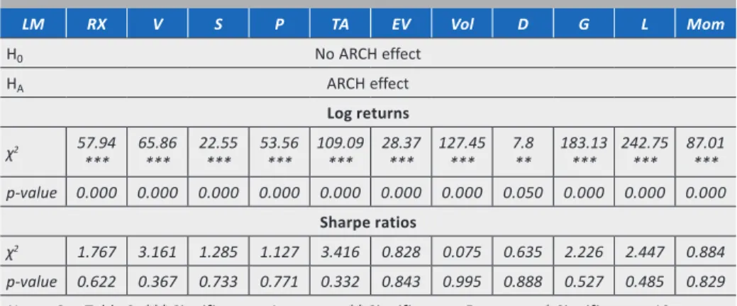
If the applicability of the GARCH models is sought to be examined in a more formalised framework, Engle’s Lagrange multiplier (LM) test should be performed (“ARCH effects” test). Table 3 summarises the test results.
Table 3
Engle’s ARCH effect test for market portfolio’s and pure factor portfolios’ returns with 3 weeks lag
LM RX V S P TA EV Vol D G L Mom
H0 No ARCH effect
HA ARCH effect
Log returns χ2 57.94
*** 65.86
*** 22.55
*** 53.56
*** 109.09
*** 28.37
*** 127.45
*** 7.8
** 183.13
*** 242.75
*** 87.01
***
p-value 0.000 0.000 0.000 0.000 0.000 0.000 0.000 0.050 0.000 0.000 0.000 Sharpe ratios
χ2 1.767 3.161 1.285 1.127 3.416 0.828 0.075 0.635 2.226 2.447 0.884 p-value 0.622 0.367 0.733 0.771 0.332 0.843 0.995 0.888 0.527 0.485 0.829 Notes: See Table 2. *** Significant at 1 per cent, ** Significant at 5 per cent, * Significant at 10 per cent
When examining the log returns, the H0 hypothesis can be rejected in the case of the Russell 3000 Index and most of the factors at rational significance levels, so the ARCH effect can be observed. The dividend factor is not significant at 1 per cent, but it is only just so at 5 per cent. The analysis of the Sharpe ratios shows that no ARCH effect can be observed for any factor, so the H0 hypothesis cannot be rejected. If the Sharpe ratios were shown as in Figure 2, it would be clear that there is no substantial volatility clustering. Based on the results, the performance of the Sharpe ratios is tested with a simple OLS regression. Since no autocorrelation can be observed, the next task is to determine the heteroscedasticity of the error terms. The relevant Breusch–Pagan (BP) test can be found in Table 4.
Table 4
Heteroscedasticity test of the factor portfolios’ Sharpe ratios
BP V S P TA EV Vol D G L Mom
H0 Constant variance
H1 Heteroscedasticity
χ2 9.58
*** 0.43 0.09 12.67
*** 3.15
* 5.75
** 37.60
*** 12.32
*** 18.22
*** 2.36 p-value 0.002 0.512 0.766 0.000 0.076 0.017 0.000 0.000 0.000 0.125 Notes: See Table 2. *** Significant at 1 per cent, ** Significant at 5 per cent, * Significant at 10 per cent
At the usual significance level of 5 per cent, the H0 hypothesis cannot be rejected in the case of the size, profitability, earnings variability and momentum factors, so the error terms of these factors are assumed to be homoscedastic. Based on the BP test, the residual variables of the other factors are heteroscedastic, and therefore the robust version of the OLS regression is used in their case.
7. Empirical findings
This section of the paper presents the empirical findings of the analysis. The hypotheses are as follows:
Hypothesis 1: The given pure factor portfolio produced excess returns over the passive strategy.
In formal terms:
H0: RP (factor) = MRP, or β0 = 021 HA: RP (factor) ≠ MRP, or β0 ≠ 0
Hypothesis 2: The given pure factor portfolio produced risk-adjusted excess return over the passive strategy.
In formal terms:
H0: Sharpe (factor) = Sharpe (passive strategy) HA: Sharpe (factor) ≠ Sharpe (passive strategy)
21 RP and MRP are short for the risk premium and market risk premium over the risk-free rate, respectively.
The risk-free rate is the return on the 1-month US T-bill for the given period.
In the regression methodology, Jensen’s alpha equals the intercept, which is usually denoted as β0. In the literature on investments, alpha is actually a “special” β0.
The above hypotheses are actually the tests of the market anomalies presented in the section on literature review, but they can also be interpreted as the tests of efficient markets. The hypotheses are examined for the entire period under review (2000–2018), the crisis years (2000–2009) and the recovery period after the crisis (2009–2018). The division of the entire period into phases practically adds a subhypothesis to the main ones: Is it possible to achieve risk-adjusted excess return over the market with the factors in the crisis (recovery) years?
The first hypothesis assesses Jensen’s alpha; it is tested using the DCC GARCH model, the regression model based on conditional variances and covariances. The second hypothesis tests the Sharpe ratio. To verify the Sharpe ratio hypotheses, the OLS regression model handling heteroscedasticity is used in the case of the factors where this is necessary (otherwise the calculations are based on the traditional OLS).
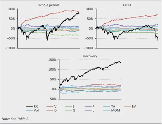
Before the detailed analysis of the results of the regression calculations, the performance of the factors and the market portfolio in the past 19 years should be evaluated. Figure 3 shows the cumulative log returns of the Russell 3000 Index and the ten factor portfolios based on weekly data. The crisis and the recovery years are distinguished, and the total 19-year cumulative return series is also shown.
The examination of the entire period attests that the performance of the market index (RX) (black solid line) basically caught up with the value factor by the end of 2018 (V line). During the crisis, the value factor performed better than all the other strategies and the market as a whole. In this period, the cumulative return of the pure factors exceeded the return of the market portfolio several times. The last ten years heralded a change, and the market return was much higher than the factor returns.
Figure 3 may suggest that the factor portfolios are less volatile than the market portfolio. This is precisely because of the structure of pure factor portfolios:
they control for the effects of other factors, making the actual return–standard deviation relationship easier to capture, and thus also reducing standard deviation (see Menchero – Lee 2015:83 and Clarke et al. 2017:27). In connection with the relationship between total market risk and the volatility of the various factors, the paper by Csóka et al. (2009) should be mentioned. The authors acknowledge in their article that risk can always be allocated in a stable manner, so that no subset (coalition) of the subelements (factors) resists the given allocation.
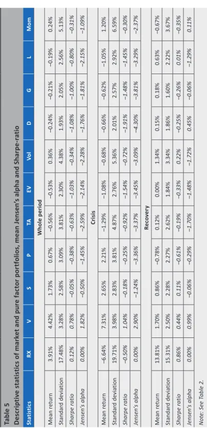
Table 5 contains the average return and standard deviation of the factors and the market in recent years as well as the performance measures. The average return and standard deviation figures are annual values calculated from weekly log returns.22
22 The calculation methodology is as follows (for the more detailed relationships between the formulas, see Medvegyev – Száz 2010:15–17): the arithmetic average of the weekly log returns – ln(St/St-1) – gives the average weekly log return (rh), and the standard deviation of the weekly log returns (σh) is also obtained.
The annual average log return is calculated from the formula “r = rh * 52”, while the annual average standard deviation is derived from “σ = σh * √52”. The average annual Sharpe ratio is derived by substituting the annualised returns and the annualised standard deviation into formula (15). The average annual Jensen’s alpha is the output of the GARCH regression (the regression calculates the average weekly alpha, which has to be multiplied by 52 to give the average annual alpha).
Figure 3
Cumulative logreturns of Russell 3000 Index and pure factor portfolios between 2000 and 2018
Whole period 100%
50%
0%
–50%
–100%
100%
50%
0%
–50%
–100%
150%
100%
50%
0%
–50%
Crisis
Recovery
RX V
Vol LP
S MOM
D EV
G TA
Note: See Table 2.
Table 5 Descriptive statistics of market and pure factor portfolios, mean Jensen’s alpha and Sharpe-ratio StatisticsRXVSPTAEVVolDGLMom Whole period Mean return3.91%4.42%1.73%0.67%–0.56%–0.53%0.36%–0.24%–0.21%–0.19%0.24% Standard deviation17.48%3.28%2.58%3.09%3.81%2.30%4.38%1.93%2.05%2.56%5.13% Sharpe ratio0.12%0.78%–0.05%–0.38%–0.63%–1.03%–0.34%–1.08%–1.00%–0.80%–0.31% Jensen’s alpha0.00%1.82%–0.50%–1.45%–2.59%–2.14%–2.28%–1.76%–1.81%–2.15%–1.09% Crisis Mean return–6.64%7.31%2.65%2.21%–1.29%–1.08%–0.68%–0.66%–0.62%–1.05%1.20% Standard deviation19.71%3.98%2.83%3.81%4.87%2.76%5.36%2.01%2.57%2.92%6.59% Sharpe ratio–0.50%1.04%–0.18%–0.25%–0.92%–1.54%–0.72%–1.91%–1.48%–1.45%–0.30% Jensen’s alpha0.00%2.90%–1.24%–3.36%–3.37%–3.45%–3.09%–4.30%–3.81%–3.29%–2.37% Recovery Mean return13.81%1.70%0.86%–0.78%0.12%0.00%1.34%0.15%0.18%0.63%–0.67% Standard deviation15.31%2.50%2.28%2.27%2.62%1.84%3.34%1.86%1.60%2.22%3.67% Sharpe ratio0.86%0.44%0.11%–0.61%–0.19%–0.33%0.22%–0.25%–0.26%0.01%–0.35% Jensen’s alpha0.00%0.99%–0.06%–0.29%–1.70%–1.48%–1.72%0.45%–0.06%–1.29%0.11% Note: See Table 2.
The examination of the entire period (2000–2018) shows that the value factor had the highest returns (4.42 per cent). Positive returns could also be achieved with the passive strategy (3.91 per cent), the small firm factor (1.73 per cent), the profit factor (0.67 per cent) as well as the volatility (0.36 per cent) and the momentum factor (0.24 per cent). When adjusting for risk (Sharpe ratio), the best performance is still linked to the value factor (0.78 per cent, compared to 0.12 per cent by the market), while the performance of the profitability, small firm, volatility and momentum factors is negative. The average annual return of the other factors was slightly negative.
In the “crisis” period (between 2000 and 2009), positive returns could be achieved with the value (7.31 per cent), the size (2.65 per cent), the profit (2.21 per cent) and the momentum factor (1.20 per cent). The passive strategy fared fairly poorly (–6.64 per cent). It can be seen that although the returns of the other factors were negative, the losses were always lower than in the case of the market factor. All in all, the crisis years saw higher volatility than the entire period under review, and therefore the Sharpe ratios are negative everywhere, except for the value factor.
In the “growth” years (between 2009 and 2018), returns were positive with decreasing volatility, except for the profit, momentum and earnings variability factor. Nonetheless, the positive returns were mostly close to zero. At this time, the market portfolio outperformed the factor portfolios by far, generating a return of 13.81 per cent, compared to the average annual performance of 0.35 per cent in the case of the factors.
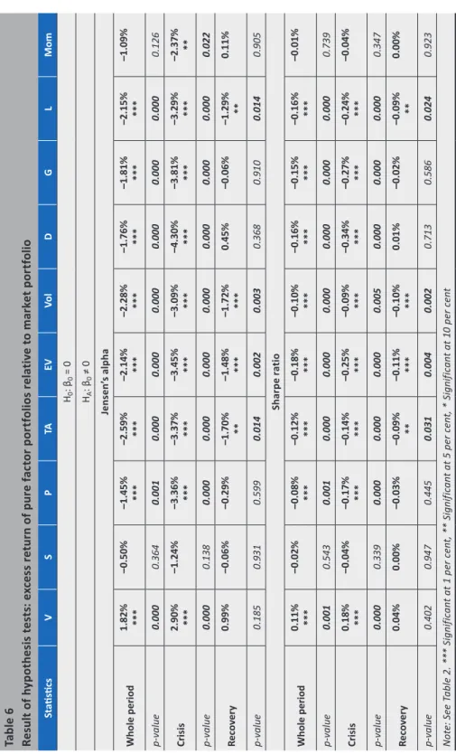
Table 6 contains the outcome of hypothesis testing of excess return. We can say that the two types of performance measures basically lead to the same conclusions;
therefore, only Jensen’s alpha is analysed below.