Control of a Uniform Step Asymmetrical 9-Level Inverter Based on Artificial Neural Network Strategy

Control of a Uniform Step Asymmetrical 9-Level Inverter Based on Artificial Neural Network Strategy

Rachid Taleb

, Abdelkader Meroufel

, Patrice Wira

1Electrical Engineering Department, Hassiba Ben Bouali University BP 151 Hay Es-Salam Chlef, Algeria, e-mail: murad72000@yahoo.fr

2Intelligent Control and Electrical Power Systems Laboratory (ICEPS) Djillali Liabes University, BP 89 Sidi Bel-Abbes, Algeria

3Laboratoire Modélisation, Intelligence, Processus et Systèmes (MIPS) Université de Haute Alsace, 68093 Mulhouse, France

Abstract: A neural implementation of a harmonic elimination strategy for the control a uniform step asymmetrical 9-level inverter is proposed and described in this paper. A Multi-Layer Perceptrons (MLP) neural network is used to approximate the mapping between the modulation rate and the required switching angles. After learning, the neural network generates the appropriate switching angles for the inverter. This leads to a low- computational-cost neural controller which is therefore well suited for real-time applications. This neural approach is compared to the well-known Multi-Carrier Pulse- Width Modulation (MCPWM). Simulation results demonstrate the technical advantages of the neural implementation of the harmonic elimination strategy over the conventional method for the control of an uniform step asymmetrical 9-level inverter. The approach is used to supply an asynchronous machine and results show that the neural method ensures a highest quality torque by efficiently canceling the harmonics generated by the inverter.

Keywords: Uniform step asymmetrical multilevel inverter, Harmonics Elimination Strategy, Artificial Neural Networks, Multi-Layer Perceptron, Multi-Carrier Pulse-Width Modulation

1 Introduction

Inverters are widely used in modern power grids; a great focus is therefore made in different research fields in order to develop their performance. Three-level inverters are now conventional apparatus but other topologies have been attempted this last decade for different kinds of applications [1]. Among them, Neutral Point Clamped (NPC) inverters, flying capacitors inverters also called imbricated cells, and series connected cells inverters called cascaded inverters [2].

This paper is a study about a three-phase multilevel converter based on series connected single phase inverters (partial cells) in each phase. A multilevel converter with k partial inverters connected in serial is presented by Fig. 1. In this configuration, each cell of rank j = 1, ...k is supplied by a dc-voltage source udj. It has been shown that feeding partial cells with unequal dc-voltages (asymmetric feeding) increases the number of levels of the generated output voltage without any supplemental complexity to the existing topology [3]. These inverters are referred to as ”Asymmetrical Multilevel Inverters” or AMI.

+

-

ud1

+

-

ud2

+

-

udk

+

-

ud1

+

-

ud2

+

-

udk

+

-

ud1

+

-

ud2

+

-

udk

O

a b c

Figure 1

Three-phase structure of a multilevel converter with k partial monophased inverters series connected per phase

Some applications such as active power filtering need inverters with high performances [4]. These performances are obtained if there are still any harmonics at the output voltages and currents. Different Pulse-Width Modulation (PWM) control-techniques have been proposed in order to reduce the residual harmonics at the output and to increase the performances of the inverters [5]. The most popular one is probably the multi-carrier PWM technique [6] which shifts the harmonics to high frequencies by using high-frequency carriers. However, electronic devices and components have limited switching-frequencies. High- frequency carriers are therefore limited by this constraint. An alternative solution consists in adapting the principle of the Harmonics Elimination Strategy (HES) to AMIs [7]. The HES allows canceling the critical harmonic distortions and therefore controlling the fundamental component of the signal by using electronic devices with low switching frequencies.

The principle of this technique relies on the resolution of a system of non linear equations to elaborate the switching angle control signals for the electronic devices [8]. Practically, the implementation of this method requires memorizing

all the firing angles which is complex and needs considerable computational costs.

Mathematical solutions with limited computational costs are therefore preferably used for real-time applications. The approach can be achieved with Artificial Neural Networks (ANNs) which are known as parsimonious universal approximators. Their learning from examples leads to robust generalization capabilities [9].

This paper proposes a HES based on ANNs to control a 9-level Uniform Step Asymmetrical Multilevel Inverter (USAMI). The work presented in [10] has been applied to an 11-level USAMI. In this paper, the neural implementation of the HES is applied to 9-level USAMI. Standard Multi-Layer Perceptrons (MLP) [11]

are used for approximating the relationship between the modulation rate and the inverters switching angles. The performance of this neural approach is evaluated and compared to the MCPWM technique. The proposed neural strategy is also evaluated when the inverter supplies an asynchronous machine. In this application, it is important that the implemented controller computes appropriate switching angles for the inverters in order to minimize the harmonics absorbed by the asynchronous machine. Performances where successfully achieved, the neural controller demonstrates a satisfying behavior and a good robustness.

The paper is organized as follows. USAMIs are described and modeled in Section 2. Section 3 briefly introduces the well-known MCPWM and brings out the original HES based on a MLP. Section 4 evaluates the proposed neural strategy in computing optimal angles of an inverter used to supply an asynchronous machine.

The results show that the neural method cancels the harmonics distortions and supplies the machine with a well-formed sinusoidal voltage waveform. Finally, a summary of the results is presented in the Conclusion.

2 Uniform Step Asymmetrical Multilevel Inverters

Multilevel inverters generate at the ac-terminal several voltage levels as close as possible to the input signal. Fig. 2 for example illustrates the N voltage levels us1, us2, ... usN composing a typical sinusoidal output voltage waveform. The output voltage step is defined by the difference between two consecutive voltages. A multilevel converter has a uniform or regular voltage step, if the steps ∆u between all voltage levels are equal. In this case the step is equal to the smallest dc-voltage, ud1 [6]. This can be expressed by

1 )

1 ( 2

3 1

2 s s s ... sN sN d

s u u u u u u u

u − = − = = − − =Δ = (1)

If this is not the case, the converter is called a non uniform step AMI or irregular AMI. An USAMI is based on dc-voltage sources to supply the partial cells (inverters) composing its topology which respects to the following conditions [6]:

⎪⎩

⎪⎨

⎧ +

≤

≤

≤

≤

∑

= 1 1 2 1

2 1

...

j l

dl dj

dk d

d

u u

u u

u

(2)

where k represents the number of partial cells per phase and j = 1, ...k. The number of levels of the output voltage can be deduced from

∑

+

= ^k

j

udj

N

1

2

1 (3)

This relationship fundamentally modifies the number of levels generated by the multilevel topology. Indeed, the value of N depends on the number of cells per phase and the corresponding supplying dc-voltages.

θ1 θ2 θp

π/2

π 2π

3π/2 us

us1

us2

usN

us(N-1)

…

…

..…

Figure 2

Typical output voltage waveform of a multilevel inverter

Equation (3) accepts different solutions. With k = 3 for example, there are two possible combinations of supply voltages for the partial inverters in order to generate a 11-level global output, i.e., (ud1, ud2, ud3) ∈ {(1, 1, 3); (1, 2, 2)}, and there are three possible combinations to generate a 15-level global output, i.e., (ud1, ud2, ud3) ∈ {(1, 1, 5); (1, 2, 4); (1, 3, 3)}. Fig. 3 shows the possible output voltages of the three partial cells of the 9-level inverter with k = 3. The dc-voltages of the three cells are ud1 = 1p.u., u_d2 = 1p.u. and u_d3 = 2p.u. The output voltages of each partial inverter are noted up1, up2 and up3 and can take three different values:

up1 ∈ {−1, 0, 1}, u_p2 ∈ {−1, 0, 1} and u_p3 ∈ {−2, 0, 2}. The result is a generated output voltage with 9 levels: us ∈ {−4, −3, −2, −1, 0, 1, 2, 3, 4}. Some levels of the output voltage can be generated by different commutation sequences. For example, there are four possible commutation sequences resulting in us= 2p.u.:

(up1, up2, up3) ∈ {(−1, 1, 2); (0, 0, 2); (1, −1, 2); (1, 1, 0)}. These redundant combinations can be selected in order to optimize the switching process of the inverter [12].

Parcial cells us = up1 + up2 + up3

(0) 1 2 3

up2 + up3

up3

up2

4 3 2 1 0 -1 -2 -3 -4

Figure 3

Possible output voltages of each partial inverter to generate N = 9 levels with k = 3 cells per phase (with ud1 = 1p.u., ud2 = 1p.u. and ud3 = 2p.u.)

These different possibilities offered by the output voltage of the partial inverters, and the redundancies among them to deliver a same output voltage level, can be considered as degrees of freedom which can be exploited in order to optimize the use of a AMI.

3 Multilevel Inverters Control Strategies

Several modulation strategies have been proposed for symmetrical multilevel converters. They are generally derived from the classical modulation techniques used for more traditional converters [12]. Among these methods, the most common used is the multi-carrier sub-harmonic PWM technique. This modulation method can also be used to control asymmetrical multilevel power converters. In the case of AMIs, other kinds of modulation can be used [3].

In this Section, we briefly introduce the MCPWM technique. We also propose a HES based on ANNs. These control strategies will be compared by computer simulations. The objective is to elaborate optimized switching angles for an 9- level USAMI. The inverter is then employed to supply an asynchronous machine.

3.1 Multi-Carrier PWM (MCPWM)

The principle of the MCPWM is based on a comparison of a sinusoidal reference waveform with vertically shifted carrier waveforms. N − 1 carriers are required to generate N levels. As shown in Fig. 4, the carriers are in continuous bands around the reference zero. They have the same amplitude Ac and the same frequency fc. The sine reference waveform has a frequency fr and an amplitude Ar. At each

instant, the result of the comparison is 1 if the triangular carrier is greater than the reference signal and 0 otherwise. The output of the modulator is the sum of the different comparisons which represents the voltage level. The strategy is therefore characterized by the two following parameters [6], respectively called the modulation index and the modulation rate:

r c

f

m= f (4)

c r

A A r N

1 2

= − (5)

0 0.002 0.004 0.006 0.008 0.01 0.012 0.014 0.016 0.018 0.02 -1

-0.8 -0.6 -0.4 -0.2 0 0.2 0.4 0.6 0.8 1

Figure 4

Multi-carrier PWM generation for N = 9 levels (with m = 24 and r = 0.8)

We propose to develop a 9-level inverter composed of k = 3 partial inverters per phase with the following dc-voltage sources: ud1 = 1p.u., ud2 = 1p.u. and u_d3 = 2p.u.. The output voltage Vab and its frequency representation are respectively presented by Fig. 5 and Fig. 6. The output voltages up1, up2 and up3 of each partial inverter and the resulting voltage for the first phase are represented by Fig. 7.

Vab ( p.u.)

time (s)

0 0.002 0.004 0.006 0.008 0.01 0.012 0.014 0.016 0.018 0.02 -6

-4 -2 0 2 4 6

Figure 5

Output voltage Vab of the 9-level USAMI controlled by the MCPWM (with m = 24 and r = 0.8)

0 10 20 30 40 50 60 70 0

1 2 3 4 5 6

Amplitude (p.u.)

harmonic ranks harmonic of rank 2 harmonic of rank 4 fundamental companent

THD = 9.19 %

Figure 6

Frequency content of the output voltage Vab with the MCPWM strategy (with m = 24 and r = 0.8)

up1 ( p.u.)

-1 0 1

up2 ( p.u.)

-1 0 1

up3 ( p.u.)

-2 0 2

Va ( p.u.) =up1 + up2 + up3

time (s)

0 0.002 0.004 0.006 0.008 0.01 0.012 0.014 0.016 0.018 0.02 -4

-3 -2 -1 0 1 2 3 4

Figure 7

Output voltages of each partial inverter and total output voltage Va of the 9-level USAMI controlled by the MCPWM (with m = 24 and r = 0.8)

3.2 Harmonics Elimination Strategy with ANNs

A) Harmonics Elimination Strategy (HES): The HES is based on the Fourier analysis of the generated voltage us at the output of the USAMI (see Fig. 2) [13].

This voltage is symmetric in a half and a quarter of a period. As a result, the even harmonic components are null. The Fourier series expansion for the us voltage is thus:

⎪⎪

⎩

⎪⎪⎨

⎧

=

=

∑

∑

=

∞

= p i d i n

n n s

n n u u

t n u u

1 1 1

4 cos sin π θ

ω

(6)

where un represents the amplitude of the harmonic term of rank n, p = (N − 1)/2 is the number of switching over a quarter of a period, and θ_i are the switching angles (i = 1, 2...,p).

The p switching angles in (6) are calculated by fixing the amplitude of the fundamental term and by canceling the p − 1 other harmonic terms. Practically, four switching angles (θ₁, θ₂… θ₄) are necessary for canceling the three first harmonics terms (i.e., harmonics with a odd rank and non multiple of 3, therefore 5, 7 and 11) in the case of a three phase 9-level USAMI composed of k = 3 partial inverters per phase supplied by the dc-voltages ud1 = 1p.u., ud2 = 1p.u. and u_d3 = 2p.u. These switching angles can be determined by solving the following system of non linear equations:

{ }

⎪⎪

⎩

⎪⎪⎨

⎧

∈

=

=

∑

∑

=

= 4 1 4

1

11 , 7 , 5 for 0 cos cos

i

i i

i

n n

r θ

π θ

(7)

where r = u1/4ud1 is the modulation rate. The solution of (7) must also satisfy

4 2

3 2

1 θ θ θ π

θ < < < < (8)

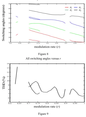
and can be solved by applying the Newton-Raphson method. This method returns all the possible combinations of the switching angles for different values of r. The result is represented by Fig. 8 where one can see the presence of two possible solutions of angles for 0.70 ≤ r ≤ 0.76. On the other side, the system does not accept any solution for r < 0.629, 0.64 < r < 0.7 and 0.897 < r < 0.921. The system has an unique solution for all the other values of r.

In the case of two possible solutions for an angle θi, the criteria for selecting one of them can be the Total Harmonic Distortion (THD). The best angle values are therefore the ones leading to the lowest THD. The THD is a quantifiable expression for determining how much the signal has been distorted. The greater

are the amplitudes of the harmonics, the greater are the distortions. The THD is defined by:

∑

∑ ∑

=

∞

=

=

= ⎟⎟

⎠

⎞

⎜⎜

⎝

= ⎛ ⁴

1 2

4 2

1

cos

1 cos ^p

i i n

p i

n i

THD n θ θ (9)

This is shown in Fig. 9 corresponding to the solutions given in Fig. 8. Choosing the switching angles based on this criteria, the multiple switching angle solutions given in Fig. 8 reduce to the single set of solutions given in Fig. 10, and the corresponding THD is shown in Fig. 11.

The control of an AMI with the HES in a real-time application requires to memorize all the switching angles. A considerable computational memory space must therefore be involved for the implementation of this control law.

0.6 0.65 0.7 0.75 0.8 0.85 0.9 0.95 1

10 20 30 40 50 60 70 80 90

θ3

θ4

θ1

θ2

Switching angles (degrees)

modulation rate (r)

Figure 8 All switching angles versus r

0.6 0.65 0.7 0.75 0.8 0.85 0.9 0.95 1

5 6 7 8 9 10 11 12 13 14

THD (%)

modulation rate (r) Figure 9

THD versus r for all switching angles

0.6 0.65 0.7 0.75 0.8 0.85 0.9 0.95 1 10

20 30 40 50 60 70 80 90

θ3

θ4

θ1

θ2

Switching angles (degrees)

modulation rate (r)

Figure 10

Switching angles versus r leading to the lowest THD

THD (%)

modulation rate (r)

0.6 0.65 0.7 0.75 0.8 0.85 0.9 0.95 1

5 6 7 8 9 10 11 12 13 14

Figure 11

THD versus r for the switching angles that result in the lowest total harmonic distortion

B) Application of ANNs: ANNs have gained increasing popularity and have demonstrated superior results compared to alternative methods in many studies.

Indeed, ANNs are able to map underlying relationship between input and output data without prior understanding of the process under investigation. This mapping is achieved by adjusting their internal parameters called weights from data. This process is called the learning or the training process. Their interest comes also from their generalization capabilities, i.e., their ability to deliver estimated responses to inputs that were not seen during training. Hence, the application of ANNs to complex relationships and processes makes them highly attractive for different types of modern problems [9, 14].

We use a neural network to learn the switching angles previously provided by the Newton-Raphson method. The approach aims to replace the painful memorization of the angles in order to make its implementation realizable in a real-time application. MLPs [11] are well suited for this task. Associated to the backpropagation learning rule, they are known as universal approximators [9].

An MLP network is composed of a number of identical units called neurons organized in layers, with those on one layer connected to those on the next layer

(except for the last layer or output layer). Indeed, MLPs architecture is structured into an input layer of neurons, one or more hidden layers and one output layer.

Neurons belonging to adjacent layers are usually fully connected and the activation function of the neurons is generally sigmoidal or linear. In fact, the various types and architectures are identified both by the different topologies adopted for the connections and by the choice of the activation function.

Some parameters of ANNs can not be determined from an analytical analysis of the process under investigation. This is the case of the number of hidden layers and the number of neurons belonging to them. Consequently, they have to be determined experimentally according to the precision which is desired for the estimation. The number of inputs and outputs depends from the considered process. In our application, the MLP has to map the underlying relationship between the modulation rate (input) and the p switching angles (output). The MLP shown in Fig. 12 is composed by one input neuron and p output neurons.

θ₁(l)

θ_p(l) r(l)

Input Layer (one neuron)

Hidden Layer (m neurons)

Output Layer (p neurons)

Figure 12

Multi-Layer Perceptron network topology (1 × m × p) used to generate switching angles

The MLP must be trained in order to adjust and to find the adequate weights. This is achieved by using probabilistic learning techniques and with data from the process under investigation. The training data consists of the inputs R and the corresponding desired output vectors S:

[

]

R= … … (10)

[ ]

⎥⎥

⎥

⎦

⎤

⎢⎢

⎢

⎣

⎡

=

=

) ( )

( )

1 (

) ( )

( )

1 ( ) ( ) ( ) 1 (

1 1

1

n l

n l

n S l S S S

p p

p θ θ

θ

θ θ

θ

…

… (11)

In the last two expressions, l = 1... n, where n is the number of examples. For a given input r(l), the MLP computes an estimated output vector

l T θ l θ l

Sˆ()=[ˆ₁() … ˆ_p()] that must be as close as possible to the ideal desired output S(l). The difference E(l)=(Sˆ(l)-S(l))² constitutes the squared output error for example l that is used by the training algorithm to correct the weights of the

neurons. This is repeated for the n samples composing the training data set until convergence is reached. The learning is achieved with the backpropagation algorithm [9].

After the training process, the MLP is able to estimate the angles corresponding to an input r(l). In other words, the MLP has learned the functions θi = fi(r) with i = 1... 4. By approximating these functions, the MLP will be able to deliver the angles for the real-time control of the inverter.

4. Results

4.1 Learning Performance

The most significant harmonics in power systems are those of rank 5, 7 and 11.

These harmonics are essentially present at the output of the USAM. We therefore chose to use explicitly cancel them with the MLP-based approach. The learning is elaborated with the Newton-Raphson method and the optimal angles are the ones resulting in the lowest THD when several solutions exist.

A MLP with one hidden layer is used with a training set composed of n = 33 examples. The MLP takes one input, i.e., the modulation rate, and delivers four outputs which are the switching angles. Several tests have been conducted for determining the number of neurons of the hidden layer. These tests have been achieved because there are no generally acceptable theories in the literature for choosing the number of hidden layers and hidden neurons for a specific application. The number of neurons in the hidden layers is important in the sense that it affects the learning convergence and overall generalization property of the MLP.

Table 1

Approximation errors with various sizes of the MLP Number of neurons

in the MLP layers Required iterations

Learning error (degrees)

1 × 2 × 4 10 000 4.372

1 × 4 × 4 10 000 3.213

1 × 6 × 4 10 000 2.105

1 × 7 × 4 10 000 1.467

1 × 8 × 4 8 943 0.893

1 × 9 × 4 6 671 0.677

1 × 10 × 4 4 249 8 10^-2

1 × 11 × 4 2 637 4 10^-3

1 × 12 × 4 1 528 1 10^-3

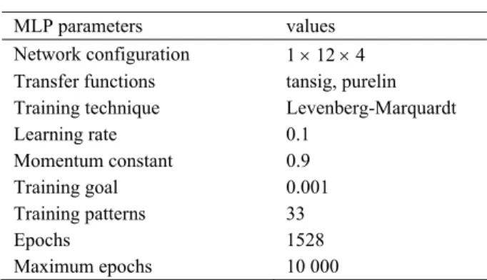
Results are provided by Table 1. According to this table, a MLP with 12 neurons in the hidden layer has been adopted. The approximating error remains the same with 12 neurons as with a higher number of neurons in the hidden layer. This configuration has been chosen after different experiments, it represents the best compromise between computational costs and performances. The other parameters of the MLP are detailed in Table 2.

Table 2 Properties of the MLP

MLP parameters values

Network configuration 1 × 12 × 4 Transfer functions tansig, purelin Training technique Levenberg-Marquardt

Learning rate 0.1

Momentum constant 0.9

Training goal 0.001

Training patterns 33

Epochs 1528

Maximum epochs 10 000

The learning convergence of the 1×12×4-MLP is reached after 1528 epochs, and leads to angle errors less than 0.001 degrees. The outputs delivered by the MLP are therefore very close to the angles given by the Newton-Raphson method. The estimated angles are represented by Fig. 13. The evolution of the training Sum- Squared-Error (SSE) is shown by Fig. 14.

0.6 0.65 0.7 0.75 0.8 0.85 0.9 0.95 1

10 20 30 40 50 60 70 80 90

θ3

θ4

θ1

θ2

Switching angles (degrees)

modulation rate (r) Figure 13

Switching angles versus r estimated by the MLP (•) and calculated with Newton-Raphson method (−)

Sum-Squared Error

epoch

0 500 1000 1500

10^-4 10^-3 10^-2 10^-1 10⁰ 10¹ 10² 10³ 10⁴

Figure 14 Training error

Vab ( p.u.)

time (s)

0 0.002 0.004 0.006 0.008 0.01 0.012 0.014 0.016 0.018 0.02 -6

-4 -2 0 2 4 6

Figure 15

Output voltage Vab of the 9-level USAMI controlled by the proposed neural HES (with r(l) = 0.8)

Amplitude (p.u.)

harmonic ranks

0 10 20 30 40 50 60 70

0 1 2 3 4 5 6

fundamental companent

THD = 7.66 %

harmonic of rank 13

Figure 16

Frequency content of the output voltage Vab with the proposed neural HES (with r(l) = 0.8)

up1 ( p.u.)

-1 0 1

up2 ( p.u.)

-1 0 1

up3 ( p.u.)

-2 0 2

Va ( p.u.) =up1 + up2 + up3

time (s)

0 0.002 0.004 0.006 0.008 0.01 0.012 0.014 0.016 0.018 0.02 -4

-3 -2 -1 0 1 2 3 4

Figure 17

Output voltages of each partial inverter and total output voltage Va of the 9-level USAMI controlled by the proposed neural HES (with r(l) = 0.8)

After learning, the MLP is also able to deliver the angles for inputs which were not present in the training set. Theses generalization capabilities are very interesting in our application, the neural controller is therefore always able to deliver the control signals for the inverter. For example, Fig. 15 to 17 shows the results obtained for an input which was not in the training set, r(l) = 0.8 which theoretically corresponds to θ₁ = 24.6999^o, θ₂ = 45.5307^o, θ₃ = 57.0398^o and θ₄ = 68.8887^o.

4.2 Performance in Supplying an Asynchronous Machine

In order to evaluate the performance and the robustness of the proposed approach, a 9-level USAMI is used to supply an asynchronous machine (with parameters given in the Appendix section). The neural HES is compared to the MCPWM

strategy in controlling the 9-level USAMI. The objective is to use the proposed neural strategy in order to minimize the harmonics absorbed by the asynchronous machine.

ias (A)

time (s)

0 0.1 0.2 0.3 0.4 0.5 0.6 0.7 0.8 0.9 1

-30 -20 -10 0 10 20 30

0 0.1 0.2 0.3 0.4 0.5 0.6 0.7 0.8 0.9 1

-10 0 10 20 30 40 50

0.6 0.61 0.62

9.5 10 10.5 11

Te (Nm)

time (s) Figure 18

Stator current (top) and electromagnetic torque (bottom) of the asynchronous machine fed by a 9-level USAMI controlled by the MCPWM

0 10 20 30 40 50 60 70

0 1 2 3 4 5 6

Amplitude (p.u.)

harmonic ranks harmonic of rank 2 harmonic of rank 4 fundamental companent

THD = 5.05 %

Figure 19

Frequency content of the stator current of the asynchronous machine fed by a 9-level USAMI controlled by the MCPWM

ias (A)

time (s)

0 0.1 0.2 0.3 0.4 0.5 0.6 0.7 0.8 0.9 1

-30 -20 -10 0 10 20 30

Te (Nm)

time (s)

0 0.1 0.2 0.3 0.4 0.5 0.6 0.7 0.8 0.9 1

-10 0 10 20 30 40 50

0.6 0.61 0.62

9.5 10 10.5 11

Figure 20

Stator current (top) and electromagnetic torque (bottom) of the asynchronous machine fed by a 9-level USAMI controlled by the proposed neural HES

0 10 20 30 40 50 60 70

0 1 2 3 4 5 6

Amplitude (p.u.)

harmonic ranks fundamental companent

THD = 1.92 %

Figure 21

Frequency content of the stator current of the asynchronous machine fed by a 9-level USAMI controlled by the proposed neural HES

The results of the control based on the MCPWM are presented by Figs. 18 and 19.

This first figure shows the stator current and the electromagnetic torque with significant fluctuations. The second figure shows the frequency content of the stator current. Results by using neural approach with the MLP issued for the

previous learning process are presented by Figs. 20 and 21. By comparing Fig. 19 to Fig. 21, it can be deduced that the neural HES efficiently cancels the harmonics of ranks 5, 7 and 11 from the output voltage Vab. Moreover, the amplitudes of the harmonic distortions are very small compared to the amplitude of the fundamental component.

Performances obtained with both methods are summarized in Table 3. The THD measured on Vab and resulting from the neural approach of the HES is smaller than the one obtained with the MCPWM method. The THD measured on the stator current ias is reduced by a factor 2.63 with the neural HES compared to the MCPWM method. The control is thus optimized with the neural HES in order to avoid the asynchronous machine to absorb harmonics.

Table 3

Performances of the control methods Control

method

Vab

THD (%)

ias

THD (%)

fCem

(Hz)

∆Cem

(Nm)

Nb of θ_i

MCPWM 9.19 5.05 f 1.77 2m = 48

Neural HES 7.66 1.92 2f 1.31 4p = 16

It can also be seen that the electromagnetic torque continuously oscillates at a frequency f with the MCPWM method (because of the harmonics of rank 2 and 4 which are present in the output voltage). The torque oscillates at 2f with the neural approach. The neural method also reduced the number of switching angles by a factor 3 compared to the MCPWM method which is highly appreciated for the electronic devices.

Conclusions

The performance of motors feed by inverters are closely related to the strategy used to control its supplying inverter. Indeed, the control currents of the motor can be disturbed by harmonics introduced by the inverter and Harmonics Elimination Strategies (HES) are generally used. We propose a low-cost neural implementation of a HES to control a uniform step asymmetrical 9-level inverter.

The approach is based on the learning and approximating of the relationship between the modulation rate and the switching angles with a Multi-Layer Perceptron. The resulting neural implementation of the HES uses very few computational costs. It is particularly well suited for real-time motor control tasks.

The proposed neural approach is compared to the MCPWM strategy. Simulation results are given to show the high performance and technical advantages of the neural implementation of the HES for the control of a uniform step asymmetrical 9-level inverter. The proposed neural method efficiently cancels the current harmonic distortions in supplying an asynchronous machine. As a result, the torque undulations and the switching losses are significantly reduced.

Appendix

• Supply voltages of the partial inverters with:

pu Units: ud1 = 1, ud2 = 1 and ud3 = 2;

SI Units: Ud1 = 100V, U_d2 = 100V and U_d3 = 200V.

• Asynchronous machine data:

Stator resistance Rs = 4.850Ω, Rotor resistance Rr = 3.805Ω, Stator inductance Ls

= 0.274H, Rotor inductance L_r = 0.274H, Mutual inductance L_m = 0.258H, Number of pole pairs P = 2, Rotor inertia J = 0. 031kg.m², Viscous friction coefficient Kf = 0.00136 Nm.s.rad⁻¹.

References

[1] Rodriguez, J., Lai, J. S., Peng, F.Z.: Multilevel Inverters: A Survey of Topologies, Controls, and Applications, in IEEE Transactions on Industrial Electronics, Vol. 49, No. 4, Aug. 2002, pp. 724-738

[2] Manjrekar, M. D.: Topologies, Analysis, Controls and Generalization in H- Bridge Multilevel Power Conversion, Ph.D. thesis, University of Wisconsin, Madison, 1999

[3] Mariethoz, S.: Etude formelle pour la synthèse de convertisseurs multiniveaux asymétriques: topologies, modulation et commande (in french), Ph.D. thesis, No. 3188, EPF-Lausanne, Switzerland, 2005

[4] Ould Abdeslam, D., Wira, P., Merckl, J., Flieller, D., Chapuis, Y. A.: A Unified Artificial Neural Network Architecture for Active Power Filters, in IEEE Transactions on Industrial Electronics, Vol. 54, No. 1, Feb. 2007, pp.

61-76

[5] McGrath, B. P., Holmes, D. G.: Multicarrier PWM Strategies for Multilevel Inverters, in IEEE Transactions on Industrial Electronics, Vol. 49, No. 4, Aug. 2002, pp. 858-867

[6] Song-Manguelle, J., Mariethoz, S., Veenstra, M., Rufer, A.: A Generalized Design Principle of a Uniform Step Asymmetrical Multilevel Converter for High Power Conversion, in European Conference on Power Electronics and Applications, EPE’01, Graz, Austria, Aug. 2001, pp. 1-12

[7] Taleb, R., Meroufel, A., Wira, P.: Commande par la stratégie d’élimination d’harmoniques d’un onduleur multiniveau asymétrique à structure cascade (in french), in Acta Electrotehnica, Vol. 49, No. 4, 2008, pp. 432-439 [8] Chiasson, J. N., Tolbert, L. M., McKenzie, K. J., Du, Z.: A Unified

Approach to Solving the Harmonic Elimination Equations in Multilevel Converters, in IEEE Transactions on Power Electronics, Vol. 19, No. 2, Mar. 2004, pp. 478-490

[9] Haykin, S.: Neural Networks: A Comprehensive Foundation, Prentice Hall, Upper Saddle River, N. J., 2^nd edition, 1999

[10] Taleb, R., Meroufel, A., Wira, P.: Harmonic Elimination Control of an Inverter Based on Artificial Neural Network Strategy, in 2^nd IFAC International Conference on Intelligent Control Systems and Signal Processing (ICONS 2009), Istanbul, Turkey, Sept. 2009, on CD

[11] Bishop, C. M.: Neural Networks for Pattern Recognition, Clarendon Press, Oxford, 1995

[12] Song-Manguelle, J. : Convertisseurs multiniveaux asymétriques alimentés par transformateurs multi-secondaires basse-fréquence: réactions au réseau d’alimentation (in french), Ph.D. thesis, No. 3033, EPF-Lausanne, Switzerland, 2004

[13] Dahidah, M. S. A., Agelidis, V. G.: Selective Harmonic Elimination PWM Control for Cascaded Multilevel Voltage Source Converters: A Generalized Formula, in IEEE Transactions on Power Electronics, Vol. 23, No. 4, Jul.

2008, pp. 1620-1630

[14] Khomfoi, S., Tolbert, L. M.: Fault Diagnostic System for a Multilevel Inverter Using a Neural Network, in IEEE Transactions on Power Electronics, Vol. 22, No. 3, May 2007, pp. 1062-1069