Fast three-dimensional two-photon scanning methods for studying neuronal physiology on cellular and network level

(1)

Fast three-dimensional two-photon scanning methods for studying neuronal physiology on cellular and

network level

Doctoral dissertation

Gergely Katona

Supervisor:

Dr. Balázs Rózsa PhD.

Pázmány Péter Catholic University Faculty of Information Technology

Multidisciplinary Doctoral School of Sciences and Technology

Budapest, 2014

(2)

(3)

(4)

(5)

ACKNOWLEDGEMENT

I would like to thank my friend and scientific advisor Dr. Balázs Rózsa for guiding and supporting me over the years.

Many thanks go out to co-authors and my other colleagues in our research group for their friendship and/or for the knowledge and the amazing times we spent together: Alexandra Bojdán, András Vági, Attila Kaszás, Balázs Chiovini, Botond Roska, Dániel Hillier, Dénes Pálfi, Dorina Gündisch, Ferenc Csikor, Ferenc Erdélyi, Gábor Szabó, Gábor Tamás, Gergely Szalay, Gergely Turi, Klaudia Sptizer, Linda Judák, Máté Veress, Norbert Hájos, Pál Maák, Patricia Varjú, Szabolcs Káli, Zoltán Szadai,

I am grateful to Prof. Tamás Roska, Prof. Péter Szolgay and Prof. Sylvester E. Vizi for paving the way to carry out my research at the University and at the Institute of Experimental Medicine, HAS.

This work was supported by the grants OM-00131/2007, OM-00132/2007, GOP-1.1.1-08/1- 2008-0085, NK 72959, Grant of Hungarian Academy of Sciences, French grant (TÉT_0389), Swiss-Hungarian grant SH/7/2/8, KMR_0214, FP7-ICT-2011-C 323945.

Last and most importantly, I cannot really express the level of gratitude to my Family, my wife Viki, and my sons Dani and Ádám, who were missing me during many night shifts and who were always there for me to share the good times and the hard ones as well.

In phrasing my thesis I used text from my publications (Katona et al., 2011; Katona et al., 2012) and in the introduction I also used some words of W. Denk, father of two-photon microscopy (Denk and Svoboda, 1997).

(6)

LIST OF FIGURES

Figure 1 Schematics of a two-photon microscope ... 14

Figure 2 Multiple Line Scan covering multiple ROIs. ... 17

Figure 3 The effect of benzamil on dendritic Ca²⁺ transients. ... 19

Figure 4 Roller Coaster Scanning. ... 24

Figure 5 3D two-photon dendritic imaging at 150 Hz. ... 26

Figure 6 Spontaneous and CA3 stimulation-induced subthreshold dendritic spikes. ... 28

Figure 7 Operating principle of AO deflectors... 36

Figure 8 Acousto-optical focusing. ... 37

Figure 9 Different 3D AO scanning arrangements. ... 38

Figure 10 Schematics of the 3D AO microscope setup. ... 40

Figure 11 Custom designed electronic cards for the electronic system ... 41

Figure 12 Driving functions and timing of operation of the four-deflector sequence... 43

Figure 13 3D virtual reality environment for 3D two-photon imaging. ... 44

Figure 14 Stability of 3D AO scanning in random-access mode. ... 45

Figure 15 Size of the PSF in the 3D AO scanned volume. ... 46

Figure 16 FOV of the microscope system by inspecting fluorescent beads. ... 47

Figure 17 Maximal FOV of the microscope with dynamic power compensation. ... 48

Figure 18 Three-dimensional measurement of bAPs. ... 49

Figure 19 Resolving bAPs at the sides of the FOV. ... 50

Figure 20 SNR of bAPs in the field of view. ... 51

Figure 21 Measurement of bAP propagation speed. ... 51

Figure 22 3D scanning of dendritic Ca²⁺ spike propagation in CA1 pyramidal cells. ... 53

(9)

Figure 23 In vivo image stacks of the neuronal population. ... 54

Figure 24 Automatic localization of neurons in vivo. ... 55

Figure 25 Spontaneous neuronal network activity in vivo. ... 56

Figure 26 V1 cortical neuronal network activity in vivo in response to visual stimuli. ... 57

Figure 27 Analysis of V1 cortical neuronal population activity. ... 58

Figure 28 Overview of the effect of enhancements implemented in the setup. ... 60

(10)

ABBREVIATIONS

2D – two dimensional 3D – three dimensional AO – acousto-optic AP – action potential

bAP – backpropagating action potential FOV – field of view

FWHM – full width at half maximum NCX1 – Na⁺/Ca²⁺ exchanger

NMDA – N-methyl-D-aspartate PSF – point spread function PMT – photomultiplier ROI – region of interest

SEM – standard error of the mean SNR – signal-to-noise ratio

(11)

1 INTRODUCTION

How does the brain work? This ancient question was in the focus of many clever minds in the past, from Aristotle through Szentágothai all the way to recent high profile laboratories.

However, with the development of technology new approaches could emerge. Aristotle could only rely on thinking and deduction (Gross, 1995), while with the invention of Golgi (Golgi, 1873), the novel era of neuroscience could emerge focusing on the morphology and structure of the brain. This detailed anatomical knowledge is accompanied in the recent decades with the emergence of new investigation technologies fuelling a new boom in the functional knowledge about our initial question. The revolution in this field is best underlined with the fact that in 2014 two Nobel prizes have been awarded to achievements related to functional imaging. Stefan Hell and his colleagues were awarded Nobel Prize in Chemistry because their pioneering work on superresolution fluorescent technology, STED (stimulated emission depletion), with which it is possible to study cellular processes at nanometer resolution (Hell and Wichmann, 1994; Betzig et al., 2006). Nobel prize In Physiology and Medicine was awarded for discoveries of cells that constitute a positioning system in the brain (Hafting et al., 2005). Through the work of John O'Keefe and the Moser couple this positioning system became one of the most studied high level complex network function. They used electrode arrays implanted in the brain of the animals, but we hope two-photon imaging will be able to complement these functional studies as my thesis is ultimately dedicated to make two-photon scanning also capable of neuronal network level investigations.

The systematic understanding of brain function requires methods that allow neuronal activity to be recorded at different spatial scales in three dimensions (3D) at a high temporal resolution (ideally over kHz). At single neuron level activity is differentially distributed in space and time across the dendritic and axonal segments (Rozsa et al., 2004; Johnston and Narayanan, 2008; Losonczy et al., 2008; Rozsa et al., 2008; Spruston, 2008; Katona et al., 2011). Therefore, in order to understand neuronal signal integration, activity should be simultaneously recorded at many (at least 10-100) spatial locations within the dendritic and axonal tree of a single neuron. At neuronal circuit level, closely spaced neurons can have

(12)

vastly different activity patterns (Ohki et al., 2005); on the other hand, widely separated cells may belong to the same functional circuit, influencing each other via long axonal processes. Therefore, recording techniques are required that collect information near- simultaneously (ideally measurement at all locations within a millisecond) from many cells of a neuronal population situated in an extensive volume of tissue (ideally over a cubic millimeter). Moreover, measurement should be possible on the timescales of the dendritic integration and regenerative spike propagation (Ariav et al., 2003), i.e., with sub-millisecond temporal resolution. One last aspect is that these measurements should be performed on neurons or neuronal networks which are as intact as possible, where neurons are embedded in their original tissue. This poses a challenge: cellular precision must be retained in acute brain preparations where the tissue is at least 100 µm thick or, for in vivo experiments, through millimeters of brain material.

Light microscopy is important in biological research because it enables living tissue to be observed and studied at a relatively high spatial resolution. This resolution is limited by the wavelength of light and even with superresolution technologies (Hell and Wichmann, 1994;

Betzig et al., 2006) does not rival that of electron microscopy. However electron microscopy is limited in its ability to observe living specimens (Danilatos, 1991). Other vital imaging technologies, such as MRT (magnetic resonance tomography), PET (positron emission tomography) or X-rays, can neither resolve subcellular structures nor provide high temporal resolution nor the exquisite molecular selectivity that would allow single molecules to be detected against a background of billions of others (Kerr and Denk, 2008; Kherlopian et al., 2008).

Light microscopy inside living tissues is hampered by the degradation of resolution and contrast, caused by absorption and light scattering, which is due to refractive index inhomogeneities present to a varying degree in every tissue. Deeper within the tissue, images become more degraded and high-resolution imaging eventually becomes impossible. A major step toward overcoming this problem was the invention of confocal microscopy (Amos et al., 1987; Minsky, 1988). In a confocal microscope, the illumination light is focused on a diffraction-limited spot, and this excites the sample along two cones close to the aimed focal point. Then, using the same objective, the emitted signal photons are focused onto a detector pinhole that rejects all light emitted outside of the focal point.

(13)

The main drawback of confocal microscopy is its wasteful use of both excitation and emission. On the one hand, absorption occurs throughout the specimen, but information is obtained only from a small volume around the focal point. On the other hand, light emitted from the focal point is also rejected by the pinhole if it is scattered by the tissue; this means that tissue scattering has a significant impact on the signal-to-noise ratio (SNR) of the images. This is a major problem particularly in vital fluorescence microscopy, where the limiting factors are usually either the photochemical destruction of the fluorophore (photobleaching) or the photodynamic damage to the specimen (photodamage). In confocal microscopy, only those ballistic photons that are not scattered on their way out of the tissue contribute to the signal: scattered photons, often the majority, are rejected by the detector aperture, limiting depth penetration using this technique to about 50-80 µm in brain tissue.

Excitation needs to be increased in order to compensate for this signal loss, and this further exacerbates photobleaching and photodamage. All of these problems are also found in many other, so-called single-photon excitation technologies, among them spinning-disc confocal microscopy (Petráň et al., 1968) and light sheet microscopy (Tomer et al., 2012).

Fortunately, these problems can be handled by using laser scanning microscopy in combination with two-photon excitation (Denk et al., 1990; Denk and Svoboda, 1997).

The concept of two-photon excitation is based on the idea that two photons of low energy can be combined in the same quantum event, resulting in the emission of a fluorescence photon at a higher energy than either one of the two excitatory photons. Although the probability of such absorption is extremely low, its cross section is proportional to the square of the photon flux, making it possible to counterbalance this low initial cross section by using extremely high photon fluxes. Two-photon absorption is often called nonlinear because the absorption rate is dependent on a higher-than-first-power light intensity. Such high fluxes are only present in the focus of a high numerical aperture lens illuminated by a strong, pulsed near-infrared laser.

The possibility of absorbing more than one photon during a single quantum event had been predicted more than 60 years ago (Goeppert-Mayer, 1931), but it was only confirmed experimentally after the invention of the lasers. Mode-locked lasers with a pulse duration below 1 ps and repetition rates of about 100 MHz made two-photon laser scanning microscopy feasible in practice (Denk et al., 1990).

(14)

Because the two-photon effect depend on the square of the intensity density, pulsing the laser source increases the average two-photon excitation rate compared to continuous- wave (CW) operation at the same average power. A typical Ti:sapphire laser has roughly 100 fs pulse width and 10 ns pulse repetition rate, thus it boosts the two-photon excitation rate by 100,000-fold. For the same reason, the quadratic dependence of the absorption rate on the light intensity gives two-photon microscopy its optical sectioning property because fluorescence is only generated in the vicinity of the geometrical focus where the light intensity is high. While scanning the laser focus in both lateral directions (x and y), fluorescence excitation is limited to the focal plane. No detector pinhole is necessary since – in most cases – no fluorescence is generated outside the focal volume, and all fluorescence photons, whether leaving the sample on scattered or ballistic trajectories, constitute useful signal.

The combination of low phototoxicity enabled by the single point excitation and the efficient use of fluorescence – even scattered – makes single-point two-photon microscopy a unique tool for observing function deep within the tissue; resolving small structures deeper than one millimeter in the brain (Theer et al., 2003; Helmchen and Denk, 2005;

Kobat et al., 2011). Its main drawback, however, is speed when compared to camera-based approaches where, instead of the ‘single-channel’ photomultipliers (PMTs), information can potentially be collected from millions of camera pixels simultaneously.

There are several approaches to using multi-site two-photon stimulation in combination with a camera-based detection algorithm to overcome the limitation of single-point illumination.

The simplest of these technologies is multi-beam two-photon microscopy (Niesner et al., 2007), where a string of focal spots are generated by breaking the laser beam into parallel beamlets. This causes parallel fluorescent excitation at multiple sites which are scanned to illuminate the entire focal plane. Fluorescence is detected by a high-resolution camera after imaging the focal plane onto its sensor chip. This approach makes it possible to image with a higher frame rate than with a scanned single-beam two-photon microscope, but it has one main drawback: imaging fluorescence onto the camera is sensitive to tissue scattering. As a result, this technology has about half of the penetration depth of single-point two-photon

(15)

microscopy and this – especially in the case of in vivo investigations – seriously limits its biological usability.

Recent camera-based approaches can also resolve the 3D structure of a sample by using a special light shaping microlens array (Prevedel et al., 2014) or phase mask (Quirin et al., 2014) in front of the camera combined with extended depth of field (Quirin et al., 2013) or holographic (Quirin et al., 2014) illumination. Depth information is obtained from the camera images by a computational reverse transformation which causes two major limitations. First, there is a strict limit to the number and arrangement of the regions of interest (ROIs) as they should not overlap much on the detector surface. Typically, ROIs situated at the same place but at different depths are imaged to mostly overlapping profiles on the detector surface, making it difficult to distinguish between them. Second, the imaging of the emitted light to the camera is – again – sensitive to tissue scattering, causing scattered shapes on the detector surface, challenging the reverse transformation algorithms. For example, Quirin et al., 2014 showed penetration depth of about 190 µm (3x scattering length) which is just enough to reach the first cell layers in mice in vivo, and is much less than the depths achievable by single-point two-photon microscopes.

As we have seen, a single-point two-photon microscope can reach deep structures with subcellular resolution, which makes this technology the best available tool for functional studies. However, as only one point might be illuminated at a time, special scanning methods need to be developed to sample the important biological features with enough speed to resolve their functionality. My work detailed in the next sections is dedicated to finding out and implementing such scanning methods, devices, electronics and software, and to perform cellular level biological measurements in acute brain slices and in the brain of living animals. More specifically my main aims were:

 Development of a fast scanning method for a two-photon microscope to sample sparse regions of interests effectively, e.g. to measure multiple compartments of the dendritic tree of neurons within 10 ms. (Chapter 2, Thesis 1)

 Development of a two-photon microscope capable of scanning 3D structures with high speed, e.g. to sample long tortuous dendrites with at least 100 Hz. (Chapter 3, Thesis 2)

(16)

 Development of a 3D random-access scanning capable two-photon microscope which is able to sample activity from many cells near simultaneously. (Chapter 4, Thesis 3)

(17)

2 FAST 2D REGION OF INTEREST SCANNING (THESIS 1)

In this chapter I will describe a scanning technology we developed for fast measurement of fluorescence in multiple regions selected in the focal plane. By describing this relatively simple method I will introduce some basic principles we used later in our more complex 3D technologies detailed in chapters 3 and 4.

2.1 The two-photon microscope

In a two-photon microscope (Figure 1) the laser beam used to excite the fluorescent dye is directed into the microscope via an epifluorescent light path. The excitation light is passed through a dichroic mirror to the microscope objective and is focused in the specimen. Two- photon induced fluorescence is generated only at the focal spot. Images are constructed by (raster) scanning the fluorescent volume by using a galvanometer-driven x–y scanner. The emission signal is collected by the same objective (and alternatively through the condenser) and reflected by the dichroic mirror to the detector. An additional barrier filter is needed to further attenuate the scattered excitation light. High-sensitivity detectors and electronics are used to ensure maximal detection efficiency.

The excitation light is usually a tunable mode-locked Ti:sapphire laser working at a wavelength set between 700 and 1000 nm. Fluorescent staining molecules having emission in the visible regime (500-600 nm) are used, while the dichroic mirror separates excitation and emission at about 700 nm. Optical resolution is limited by the Abbe law (modified for two photon excitation) thus it depends on the excitation wavelength and the numerical aperture of the focusing. Usually large working distance (1-3 mm) water immersion objectives are used having numerical aperture about 1, thus the lateral optical resolution is expected to be around 350-500 nm.

Galvanometers are commanded to perform raster scanning to form images and as the current commercially available scanners have a maximal driving frequency of about 2 kHz, full field images (512 x 512 pixels) can be obtained maximally at 4 frames per second speed.

(18)

We constructed a two photon microscope hosting all our improvements detailed below, for details see 2.6 Materials and methods section.

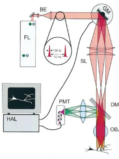
Figure 1 Schematics of a two-photon microscope

The excitation light, a train of femtosecond pulses from the mode-locked (FL) laser, passes the beam expander (BE), a pair of galvanometer scanning mirrors (GM, only one axis shown), the scan-lens (SL, essentially a low magnification eyepiece), intermediate optics inside the microscope (not shown), the objective lens (OBJ), and comes to a diffraction- limited focus inside the specimen. Some fraction of the 2-photon excited fluorescence passes back through the objective (detection of light entering the condenser or coming off to the side is possible as well) and is deflected by a dichroic mirror (DM) through a filter (blocking excitation light, not shown) into the photomultiplier detector (PMT). A computer (HAL) controls the scanners and synchronously records the signal from the PMT. Figure adopted from Denk and Svoboda, 1997.

(19)

2.2 Why region of interest scanning?

In two-photon microscopy images are traditionally obtained. These images are formed by measuring the fluorescence intensities in all pixels, moving the focal spot line-by-line;

therefore it is also called raster scanning. An ideal device to capture full images with high frame rate is the so called, resonant-galvo system. Here the mirror deflecting laser light in the x direction is mounted on a resonant scanner which is actually made of a flexible torsion mechanics and an electromotor. The motor is driven by a feedback loop making the system oscillate very fast (8 kHz in typical commercially available devices) resulting in 31 frames captured per second (512 x 512 pixels, full field) (Fan et al., 1999; Jia et al., 2010).

To record neuronal signaling and action potentials (APs) however, much larger repetition rates are necessary (ideally near kHz). To reach this goal we should give up recording entire images and instead of sampling all pixels in images we need to scan repetitively only the regions containing information for the experimenter (region of interest - ROIs).

As we measure a low number of photons (λ), the mean signal (µ) captured from a ROI and its variance (σ) follow Poisson distribution:

Equation 1.

Thus SNR is predominantly determined by the total number of photons collected from a structure within a unit time. On the other hand, the total number of photons can be written as:

Equation 2.

where η is the systems total efficiency for detecting an emitted photon (constant), ϕ is the emitted photon flux, and τ is the time spent on the ROI. Because increasing excitation in living samples quickly results in photobleaching and photodamage, we cannot increase ϕ above a certain level (determined experimentally for each sample preparation) so one can increase SNR only by increasing the time fraction spent on the ROIs.

Giving up scanning images and scanning strictly the ROIs increases the time fraction the scanner spends on the ROIs and by this ultimately increases the SNR of the information collected from the ROIs. When we select scanning lines to cover the ROIs instead of raster

(20)

scanning, total number of photons sampled from the ROI will be increased with the ratio of the time fraction spent on the ROIs during raster scanning. This is proportional to the raster scanned field of view versus the ROI area.

Equation 3.

This means that if the ROIs are small and dispersed in the (2D) field of view (FOV) – which is the usual case – one can increase SNR significantly by repetitively scanning only the information containing areas using line-scans instead of raster scanning the full (mostly not labeled) areas. The quantity of the SNR gain is dependent on the shape and extent of the ROIs, thus the geometry to be scanned.

2.3 Multiple Line Scanning

Earlier realizations could perform line-scanning only on single, straight horizontal lines which were often not matching the shape of the ROIs (Rozsa et al., 2004). We developed a system (Lorincz et al., 2007; Rozsa et al., 2008) using galvanomotor-based scanning mirrors.

These scanner motors are driven (by an appropriate closed loop driving electronics) so that their absolute position can be specified by the input analog voltage signals (see 2.6 Materials and methods). I implemented in the software that the desired regions can be drawn onto the previously made raster scanned background image. Measurement line can be constituted of multiple straight or curved line segments to cover various combinations of ROIs. These line segments can be scanned with constant speed, while intermediate sections are jumped over within 60-100 μs, using a spline interpolated path (Figure 2). We named this technology Multiple Line Scanning. Using high speed galvomotors and high performance driving electronics complex line-scans consisting of a dozen line segments can be typically performed with 100-200 Hz repetition rate, but on small straight line segments this can be tuned up to about 2 kHz.

Figure 2 shows a dendritic segment where the activity of multiple spines and their parent dendritic segment can be recorded simultaneously with Multiple Lines Scanning, resolving

(21)

individual postsynaptic events and the diffusion of Ca²⁺ between compartments.

Quantitatively the SNR gain according to Equation 3 in the case on Figure 2 (image area is 16 µm x 7 µm, ROI area is 20 µm x 0,5 µm which latter is the diameter of the PSF) results in a factor of 3,3. Another common situation is if we want to measure a 14 µm long dendritic portion caught diagonally in the field of view. With raster scanning we would need to scan a 10 by 10 µm image, thus the SNR gain according to Equation 3 (image area is 10 µm x 10 µm, ROI area is 14 µm x 0,5 µm) results in a factor of 3,8. Evaluating other likely situations of imaging dendrites, we can say that the SNR gain is approximately 3-4. Theoretically the lower extreme is 1 in the case of rectangular ROIs fully filling the raster scan; an upper extreme is if the ROI is thin, diagonal and spans the entire FOV (approximately 600 µm with a 20x objective), in this case SNR gain is 29. As raster scanning the full field of view (512 x 512 pixels; using galvanometer based scanners) is possible with only 4 Hz, we can say that the repetition rate increase is again depending on the shape and extent of the ROI, but it is between 1 and 512.

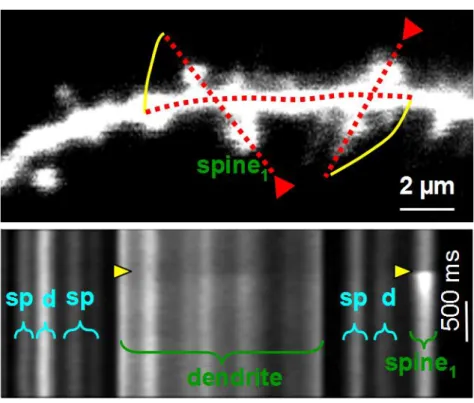
Figure 2 Multiple Line Scan covering multiple ROIs.

(Top) Multiple Line Scan drawn on a tortuous dendritic segment: two line segments cross dendritic spines and the dendrite, while the third is selected to follow the dendritic shaft linking them. (Bottom) Raw fluorescence image. Horizontal axis is space “along the line”. Spine1 receives a massive synaptic input at the time indicated by yellow triangles. As a result of Ca²⁺ diffusing

(22)

out of the spine neck a smaller, dispersed Ca²⁺ transient can also be seen in the dendritic shaft.

(Lorincz et al., 2007)

2.4 Using line-scans to investigate dendritic Ca

²⁺

dynamics

To prove the method is beneficial in biological measurements, I describe here a study we performed. Using the new method and the prototype we built we studied the role of Na⁺/Ca²⁺ exchanger (NCX1) on dendritic shafts (Lorincz et al., 2007).

In this study a major benefit of using the Multiple Line Scanning method was that by simultaneously scanning neighboring spine-dendrite pairs (Figure 2) we were easily able to isolate the cases where only single spines were activated. We used extracellular synaptic stimulation where a glass pipette is placed near (5-10 µm) the investigated dendritic segment and we tried to stimulate unlabeled axons converging onto the investigated dendrite by introducing current pulses to the pipette (see 2.6 Materials and methods). Even with carefully chosen location and current level, it is hard to selectively activate single synaptic inputs. Activation of the neighboring spines can lead to an increased Ca²⁺ influx as a result of the removal of the magnesium block of NMDA (N-methyl-D-aspartate) channel and/or the opening of voltage gated Ca²⁺ channels. Without the monitoring of neighboring synaptic activity, it cannot be excluded that the larger, previously reported Ca²⁺ signals (Mainen et al., 1999; Kovalchuk et al., 2000) are the consequence of the activation of neighboring synaptic inputs. Using our Multiple Line Scanning method we could rule out these events and study the action of NCX1s in those biologically relevant cases too, where only one synapse was activated at a time (Hiba! A hivatkozási forrás nem található.a). This results in smaller Ca²⁺signals restricted to spines and are comparable to more recent experiments, where single synaptic inputs elicited Ca²⁺ signals well compartmentalized to spines without spreading to neighboring shafts (Yuste et al., 2000).

Benzamil selectively blocks Na⁺/Ca²⁺ exchange in small concentration (30 µM) resulting in a modest effect on Ca²⁺ transients. With the improved SNR of Multiple Line Scanning we were able to significantly resolve these subtle differences in Ca²⁺ transients and therefore could show NCX1 activity in dendritic shafts and spines during repeated stimulation of single synapses (Hiba! A hivatkozási forrás nem található.b).

(23)

Figure 3 The effect of benzamil on dendritic Ca²⁺ transients.

(a) NCX1 activity does not shape Ca²⁺ transients compartmentalized to dendritic spines during single synaptic stimulation. Example average responses in the dendrite and spine in the presence (red) and absence (black) of 30 µM benzamil. (b) NCX1 activity does shape Ca²⁺

transients in dendritic shafts and spines during repeated stimulation of single synapses.

Synaptic stimulation was elicited by seven consecutive stimuli delivered at 200 Hz.

Normalized Ca²⁺ transients in a spine (Left) and parent dendrite (Right) in control conditions (black traces) and in the presence of benzamil (red traces). Traces are averages of four responses. (Lorincz et al., 2007)

We also took advantage of Multiple Line Scanning to record multiple locations with good SNR in other studies, where we studied the attenuation of backpropagating action potentials (bAPs) in interneuron dendrites (Rozsa et al., 2008; Chiovini et al., 2010).

2.5 Discussion

Multiple Line Scanning is a versatile tool which allows Ca²⁺ imaging in neuroscience on subcellular components i.e. on dendritic structures, and is capable of simultaneously recording multiple cellular processes or multiple somata, but for example it also allows blood flow measurements in capillaries. Its main benefit is increased repetition rate and SNR of the signal collection from the ROIs selected in the focal plane. The repetition rate increase compared to classical raster scanning is between 1 and 512, typically 10-100. The increase of SNR is between 1 and 29, typically 3-4. On the top of this, the technology can also be used for photostimulation with single scan head: for two-photon uncaging (Katona et al., 2011), optogenetical activation, and FRAP (fluorescence recovery after photobleaching) measurements.

(24)

2.6 Materials and methods

Electrophysiology. Pyramidal cells in the CA1 subfield of the hippocampus were visualized under 900-nm infrared differential interference contrast (DIC; 900 nm; Olympus, Budapest, Hungary). Electrodes (6–9 MΩ) were filled with 125 mM potassium gluconate, 20 mM KCl, 10 mM Hepes, 10 mM Di-Tris-salt phosphocreatine, 0.3 mM Na-GTP, 4 mM Mg-ATP, 10 mM NaCl, and 60 µM Oregon green BAPTA-1. Recordings were made at 32°C by using a MultiClamp 700B Amplifier (Axon Instruments, Foster City, CA). Cells with a resting membrane potential more negative than 65 mV were accepted. Data acquisition was performed by using pClamp8 (Axon Instruments) and a MATLAB program written in our laboratory. We used 6- to 9-MΩ patch electrodes filled with ACSF (artificial cerebrospinal fluid) for synaptic stimulation.

Two-photon imaging system. Imaging was performed by using a two-photon laser scanning system built in our laboratory. Excitation was provided by a titanium-sapphire laser (R&D Kft., Budapest, Hungary; Millennia Pro, SpectraPhysics, Fremont, CA) providing 100-fs pulses at 80 MHz at a wavelength of 805-810 nm. Focal scanning was achieved by using galvanometric scanners (VM-500; GSI Lumonics, Unterschleissheim, Germany) with a digital servo tuned for high-speed random scanning (Digital Servo; GSI Lumonics). Fluorescence was detected in the external, whole-field detection mode with photomultiplier tubes (R3896; Hamamatsu, Herrsching, Germany). Colored glass filters (BG39; CVI Technical Optics) and dichroic mirrors (750DCSX, 750DCXXR; Chroma Technology, Brattleboro, VT) were used to separate emitted fluorescence from excitation light. Position of the detectors and appropriate lenses and condenser (U-UCD8, NA = 1.4; Olympus, Budapest, Hungary) was optimized for best fluorescence collection, and the intensity of excitation laser light was also always maintained at the minimum required to attain sufficient SNR to minimize photodamage. We developed electronics and a function generator (computer card) to drive the scanner motor-directed light with high accuracy (<300 nm) along arbitrary curves at high scanning speed (>1 kHz) in the focal plane. Data recording started 20–30 min after break-in.

At the end of each experiment, a series of images across the depth of the volume encompassing the imaged neuron was taken. Measurement control, real time data acquisition, and analysis were performed with a MATLAB program developed in our laboratory. Fluorescence traces are expressed as relative fluorescence changes [ΔF/F = (F–

(25)

F⁰)/F⁰], where F⁰is the background-corrected prestimulus fluorescence. If not indicated otherwise, data are presented as means ± SEM. To get the amplitude and decay of the transients, three sweeps were averaged before and after the perfusion of benzamil at high stimulus intensities.

2.7 Thesis

Thesis 1: I developed a new method to image dendrites; by limiting the measurements only to the functionally investigated neuronal locations increased speed and signal-to-noise ratio of the measurements significantly.

Publication related to the thesis: Lorincz et al., 2007, Rozsa et al., 2008; Chiovini et al., 2010.

In two-photon microscopy the scanning is traditionally used to form images. Images are formed by measuring the fluorescence intensities in all pixels, moving the focal spot line-by- line. To record neuronal signaling and action potentials we should give up recording entire images and instead of sampling all pixels we need to scan repetitively only the regions containing interesting information for the experimenter (ROIs). This can be achieved by using galvanometer based scanning mirrors controlled by analog voltage signals boosting repetition speed to the 100 Hz - 1 kHz rate. Scanning only the interesting parts not just increases repetition speed of the measurement at a given ROI, but also increases signal-to- noise ratio (SNR) of the measured fluorescence signals, typically by a factor of 3-4. The higher the ratio of the area of the FOV to the area of the ROIs the larger the possible SNR gain is.

We developed a complex line-scanning method called Multiple Lines Scanning (Lorincz et al., 2007) and built a microscope utilizing it. We were able to use this feature to show Na⁺/Ca²⁺

exchanger (NCX1) activity in the case when multiple synaptic inputs arrive in close succession to the same dendritic branch (Lorincz et al., 2007). The major benefit of using the Multiple Line Scanning method was that by simultaneously scanning multiple neighboring spines we were able to isolate the cases where only single spines were activated. We also took advantage of this method to record multiple locations with good SNR in other studies, where we studied the attenuation of backpropagating action potentials (bAPs) in interneuron dendrites (Rozsa et al., 2008; Chiovini et al., 2010).

(26)

3 PIEZOELECTRIC OBJECTIVE POSITIONER BASED 3D SCANNING (THESIS 2)

Using scanning mirrors to deflect the laser beam enables rapid positioning of the focal point only in the focal plane of the objective. This means that ROIs whose activity we would like to measure with high speed should be within a plane perpendicular to the optical axis; hence we call these scanning methods two dimensional (2D). Biological structures are however rarely planar. Some structures such as hippocampus and the cerebellum gained their popularity because their network functionality can be well understood in slices which are cut parallel to the main connections. Measurement of other structures and even these in in vivo conditions asks for methods being able to sample activity in the 3D space. In this chapter I will detail the design of a simple system capable of performing fast 3D scanning.

Traditionally the objective is moved using a step motor driven mechanical arm which enables only slow positioning of the focal plane (Denk et al., 1990) due to the large inertia of the objective and the mechanical arm. Fast z-drive by piezo-positioners has been proposed previously (Gobel et al., 2007). In this study, authors moved the objective up and down by forcing the piezo-positioner for a sinusoidal movement. The actual phase shift and amplitude drop was compensated for in the driving signal. In this way, it was possible to resonate the objective with up to 10-20 Hz frequency, which was limited by the deviation of the objective movement from the sinusoidal function above this frequency range. In order to access 3D, Gobel et al performed spiral-scanning by using two galvo mirrors in combination with the sinusoidal objective drive to scan cellular activity within a small volume (250 x 250 x 200 µm) with about 10 Hz repetition rate.

3.1 Roller Coaster Scanning

To achieve faster scanning along a 3D trajectory we coupled to our two-photon microscope (Femto2D, Femtonics) a rapid cylindrically symmetric piezoelectric actuator (Physik Instrumente, Karlsruhe, Germany) with high resonant frequency (~ 1100 Hz without load) and used 100-700 Hz sine wave driving signal (Katona et al., 2011). Speeding up the driving

(27)

frequency of the piezo-positioner from the earlier described 10 Hz leads not just to a drop in amplitude and change in phase of the sinusoid movement (Gobel et al., 2007), but also resulted in a profound deviation of the position function from the sine wave (Figure 4A). We maintained a resonance in the objective movement without servo feedback, whilst measuring the position signal. After 50-100 cycles the movement of the objective reached a steady-state response function z(t) at a mean position (Figure 4B). We measured this non- linear z(t) function to generate a drive signal for the xy deflection (Figure 4C). First, using the z(t) response function, the t1 time was determined when the focal plane of the objective was at height z1, z(t1)=z1, (Figure 4 Ca and Cb), then at this t1 time point the xy drive signal for the galvanometer scanner was set to (x1, y1) to fit the 3D trajectory f(x1,y1,z1) (Figure 4 Cc). This process was repeated for the remaining points of the entire 3D trajectory selected for measurement.

We wrote software elements to help the fast orientation in 3D space, the selection of the 3D trajectories according to the z-stacks and the optimal utilization of the whole available z- scanning range. Namely, after acquisition of a z-stack, the recorded image series were used to aid the selection of the 3D path by scrolling through without scanning using the focusing handwheel of the microscope (rotary encoder; M101B, Megatron) for z and the computer mouse for xy coordinate settings. The selected 3D trajectory was the result of an interpolation algorithm which was based on guide points selected on the image stack of the chosen dendritic region. We named this method Roller Coaster Scanning (Katona et al., 2011) according the similarity in the movement trajectories.

The stability of the 3D trajectory scanning was verified by bleaching 3D curves in a homogeneous fluorescent plastic sample. A z-stack of the fluorescence was taken afterwards, and inverted, representing the time-averaged laser irradiation in the 3D space.

When scanning a trajectory with 150 Hz (the same as in Figure 5A) shows that the trajectory was followed at high precision in all dimensions (Figure 4D). When scanning with a much higher speed at the resonance peak around 700 Hz, the resulting bleached trajectory deviates significantly from the planned one (Figure 4E). However, the trajectory was stable;

suggesting that resonance might be better controlled with optimized mechanical design and/or with the use of software corrections. To compensate for deviations from the planned trajectory in the 150 Hz regime, we used a manual approach. We repeatedly moved the

(28)

points selecting the 3D trajectory in the xy plane while monitoring the basal fluorescence increase in the measured raw fluorescence traces until a better overlap between the 3D trajectory and the selected dendritic segment was visible.

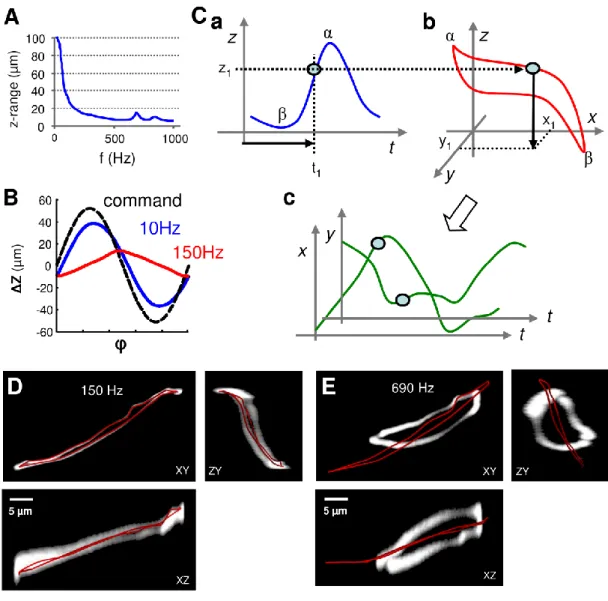
Figure 4 Roller Coaster Scanning.

(A) The z-scanning range of the Roller Coaster Scanning as a function of repetition frequency.

Note the resonance peak at 690 Hz. (B) Diagram showing the z-position of the objective as a function of time within a single oscillation period after the oscillation has become stable. The nonlinearity of the response is only apparent at higher frequencies. (C) Principle of calculating the Roller Coaster Scanning movement. (Ca) After 50-100 cycles (warm up period) the position of the objective reached a steady-state nonlinear response function (z(t)), the amplitude of which was set to be larger than the required z-scanning range in imaging. (Cb) For each t1 time-point the location on the 3D trajectory was determined whose z coordinate equaled z(t ). (Cc) The x and y coordinate projections of the 3D trajectory (x, y )

(29)

determined the x(t) and y(t) functions which were used as command signal of the digital servo of the scanner motors. As illustrated in Cb, the descending and ascending phase of the oscillation could cover different parts of the selected 3D trajectory. (D) Maximum intensity image stack projection of an originally homogeneous fluorescent sample after bleaching it along the user-selected 3D trajectory also used in Figure 5A and B. Measured intensities were inverted. User-selected 3D trajectory is overlaid in red. (E) The same measurement, but at the 690 Hz resonance peak. Note that although the measured trajectory did not follow the user selected one, it was stable suggesting that software correction is possible. On D and E scale bars apply for all panels. (Katona et al., 2011)

We tested our method in biological measurements by scanning multiple spines of a CA1 hippocampal pyramidal cell simultaneously in 3D (Figure 5A) and by scanning long segments of dendrites of a CA1 interneuron (Figure 5B). Our approach resulted in a relatively limited, but biologically relevant z-scanning range (28 µm at 150 Hz, Figure 4A), while maintaining an advantageous FOV (650 x 650 µm² with 20x objective) and resolution parameters characteristic of two-photon microscopy near the theoretical diffraction limit. Namely, we tested two objectives: in the case of XLUPlanFI 20x (Olympus) FWHM of the PSF is 450 nm in XY and 2400 nm in Z and with the LUMPlanFI/IR 60x (Olympus) FWHM of the PSF is 430 nm in XY and 2300 nm in Z. Resonation frequencies 120-200 Hz were used for the biological measurements.

To estimate a measure of the benefit of Roller Coaster Scanning in our conditions, we first constructed the length statistics of dendritic sections gained after cutting reconstructed dendritic trees into slices parallel to the focal plane (Figure 5C Inset). Then for a given slice thickness representing available z-range, we calculated the percentage of the dendritic sections being larger than a threshold, thus being appropriate for a virtual measurement (Figure 5C). To derive a simple number expressing the benefit of our new method, we compared the access rate of the ideal axial resolution z-grab condition to the 7 - 25 µm z- grab conditions used in our experiments at the mean segment length of dendrites imaged in our study (42.3 ± 7.4 μm; range, 10–250 μm). The geometric mean of the ratios representing the two extremes is approximately 27. This means that using Roller Coaster Scanning we had approximately 27 times larger chance to image 40 μm dendritic segments than it would be with 2D scanning approaches.

(30)

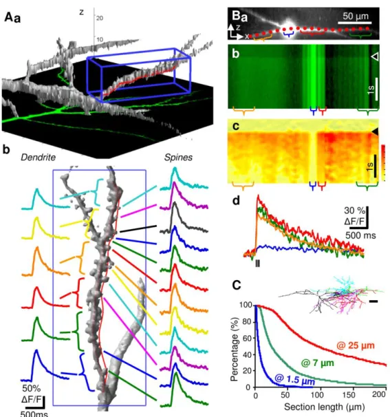
Figure 5 3D two-photon dendritic imaging at 150 Hz.

(Aa) 3D reconstruction of a CA1 pyramidal cell dendritic segment. The red curve shows the 3D trajectory of the scanning crossing the dendritic segment and spines. The blue box is 15 x 15 x 37 µm³. (Ab) Enlarged view of the blue box in Aa. A total of 18 regions including 12 spines located on the 3D scanning trajectory were measured simultaneously at 150 Hz. Ca²⁺

transients were induced by bAPs elicited by somatic current injection steps (5 APs, 35 Hz, average of 5 traces). (Ba) Maximum intensity side projection of a long CA1 interneuron dendrite. The pipette has been removed from the image. (Bb) 3D trajectory-scan measured along the dendrites in Ba. White open triangle indicates the time when bAPs were induced by somatic current injections (5 APs, 35 Hz, average of 5 traces). The horizontal axis is the spatial dimension along the measurement line (note that the scanning speed along the line is variable due to the nature of the Roller Coaster Scanning). Time is displayed along the vertical axis. (Bc) Relative fluorescence image (3D Ca²⁺ response) calculated from Bb.

(31)

Colorbar: 0-63 % ΔF/F. (Bd) Individual Ca²⁺ transients measured in the color coded regions in Bb (black bars indicate current injections). Note the high SNR. (C) Access rate of long dendritic segments for 3D scanning shown at three different z-scan ranges. (Inset) Lateral projection of six reconstructed CA1 stratum radiatum interneurons used for this statistical calculation (scale bar: 100 µm). (Katona et al., 2011)

3.2 NMDA spikes in stratum radiatum interneurons

To prove the method is beneficial in biological measurements, I describe here a study we performed on the dendrites of inhibitory interneurons. Inhibitory interneurons are considered to be the controlling units of neural networks, despite their sparse number and unique morphological characteristics when compared to excitatory pyramidal cells. Though pyramidal cell dendrites have been shown to display local regenerative events – dendritic spikes – evoked by artificially patterned stimulation of synaptic inputs (Schiller et al., 2000;

Magee and Johnston, 2005), no such studies existed for interneurons or for spontaneous events. In addition, an imaging technique needed to be developed that have the required spatial and temporal resolution for the detection of spontaneously occurring events that trigger dendritic spikes. Using Roller Coaster Scanning, we found that localized dendritic spikes can be observed in hippocampal CA1 stratum radiatum interneurons during spontaneous network activities in vitro (Figure 6). In these experiments where we searched for spontaneous dendritic spikes, slices were placed into a dual-superfusion slice chamber (the tissue slice lies on a mesh allowing flow of the perfusion fluid also under the tissue) to maintain physiologically relevant network activity (Hajos et al., 2009).

Spontaneous dendritic spikes were reproduced using synaptic stimulation and two-photon glutamate uncaging (see 3.4 Materials and methods) to be able to investigate their pharmacological properties and their dependence on the number and distribution of coincident synaptic inputs driving them. These proved dendritic spikes to be NMDA channel driven by their sensitivity to the selective blocker AP5 (D-2-Amino-5-phosphonovaleric acid), but voltage gated Na⁺ and Ca²⁺ channels did not play significant role. Simulating synaptic inputs with two-photon glutamate uncaging showed that these NMDA spikes appear when

~10 spatially clustered inputs arrive synchronously and trigger supralinear integration in relatively small (~14 µm) dynamic interaction zones (Katona et al., 2011).

(32)

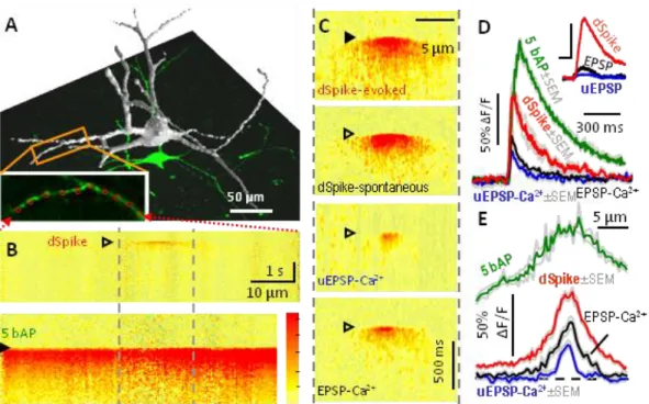
Figure 6 Spontaneous and CA3 stimulation-induced subthreshold dendritic spikes.

(A) 3D reconstruction of an interneuron. Long dendritic segments (inset) were systematically imaged to find spontaneous or CA3 stimulation-induced synaptic responses. (B) Spatially normalized 3D dendritic Ca²⁺ transients (3D Ca²⁺ responses; colorbar: 0-63% ΔF/F; dendritic length was 76 µm) showing a well compartmentalized spontaneous synaptic response (top) and a more homogeneous response evoked by 5 bAPs (bottom). (C) 3D Ca²⁺ responses representing types of spontaneous events (empty triangles) and response following CA3 stimulation (filled triangle) in a dendritic region from panel B (marked with gray dashed lines). (D) Ca²⁺ transients (average of 5-7 traces) derived at the peak of the 3D Ca²⁺

responses in B and C. Inset, Corresponding somatic membrane voltage (scale bars: 4 mV and 15 ms). (E) Spatial distribution of peak 3D Ca²⁺ responses in B and D. Gray traces show mean

± SEM (Katona et al., 2011)

3.3 Discussion

Our observations of local dendritic spikes in thin dendrites of interneurons were facilitated by more factors. We have used a new recording chamber with dual superfusion to maintain physiologically relevant network activities through better oxygen supply (see 3.4 Materials and methods). We developed Roller Coaster Scanning, increasing access rate to imaging long continuous dendritic segments. This second feature, with the preserved high spatial and temporal resolution, allowed us to precisely localize the sites and properties of spontaneous

(33)

(and evoked) individual inputs, as well as their spatially and temporally patterned combinations during integration of multiple synaptic inputs arriving onto a dendritic segment.

The optical pathway of the Roller Coaster microscope is simple, and does not contain any material beyond the objective that introduces angular or linear dispersion or laser intensity loss, therefore

 the good spatial resolution characteristic of two-photon microscopy are preserved,

 experiments requiring high energy pulses like two-photon uncaging, bleaching, ablation or in vivo imaging of deep tissue (Helmchen and Denk, 2005) are achievable

 the combination of Roller Coaster Scanning with new optical methods such as for example the already mentioned high resolution imaging technique STED is theoretically possible.

These properties make Roller Coaster Scanning ideal for scanning extensive and continuous dendritic segments with high spatial and temporal resolution.

3.4 Materials and methods

Slice preparation and electrophysiology. Acute hippocampal slices were prepared from 16- 20 day old Wistar rats using isoflurane anesthesia followed by swift decapitation, in accordance with the Hungarian Act of Animal Care and Experimentation (1998; XXVIII, section 243/1998.). Coronal (300 µm) or horizontal (450-600 μm) brain slices were cut with a vibratome and stored at room temperature in artificial cerebrospinal fluid (ACSF) (in mM:

126 NaCl, 2.5 KCl, 2 CaCl2, 2 MgCl2, 1.25 NaH2PO4, 26 NaHCO3 and 10 glucose) as previously described (Rozsa et al., 2004). The 450-600 µm thick horizontal slices were used in the experiments involving spontaneous dSpikes and were recorded in a custom-made recording chamber where improved oxygenation could be achieved by simultaneous perfusion of both the top and the bottom surfaces of the slices (Hajos et al., 2009). Preventing bubbles from entering into the recording chamber allowed long term optical measurements.

Hippocampal neurons in CA1 stratum radiatum near the border of the stratum lacunosum- moleculare were visualized using 900 nm infrared lateral illumination. Current-clamp recordings were made at 32 °C (MultiClamp 700B, Digidata 1440; Molecular Devices,

(34)

Sunnyvale, CA, USA) with glass electrodes (6–9 MΩ) filled with (in mM): 125 K-gluconate, 20 KCl, 10 HEPES, 10 Di-Tris-salt phosphocreatine, 0.3 Na-GTP, 4 Mg-ATP, 10 NaCl, 0.06 Oregon Green BAPTA-1 (OGB-1, Invitrogen) and biocytin. Cells with a resting membrane potential more negative than –50 mV were accepted.

Focal synaptic stimulation was performed by 6-9 MΩ glass electrodes filled with ACSF were placed at a distance of 10-25 µm from the dendrite (stimulation: 0.1 ms, 10-50 V, 10 ms pulse interval at double pulses; Supertech Ltd., Pécs, Hungary). Backpropagating APs were induced by somatic current injections (200–400 pA, 5 ms; 5 bAPs were evoked at 35 Hz). The NMDA receptor selective antagonist AP-5 (60 μM) was injected by a motion artifact-free rapid perfusion system as described earlier (Rozsa et al., 2008), whereas bicuculline (20 μM) was applied in the bath. All evoked EPSPs were verified for synaptic delay.

Stimulation of Schaffer collaterals at the hippocampal CA3 area (1-5 stimuli, 100 Hz, 35-65 V) was applied via the same method as used for focal synaptic stimulation, with the exception that the stimulatory pipette of 4-5 MΩ was placed in the pyramidal layer of CA3.

All chemicals and drugs unless otherwise noted were purchased from Sigma (St Louis, MO, USA). Data acquisition was performed using either pClamp8 or pClamp10 (Molecular Devices) and MES (Femtonics Ltd.) software.

Three dimensional two-photon imaging. Real-time, 3D two-photon imaging was performed using a modified two-photon microscope (Femto2D, Femtonics) enabling scanning along 3D trajectories that cross neuronal processes in 3D (Roller Coaster Scanning) using a customized piezo actuator (P726, PhysikInstrumente) for z-scanning. Resonation frequencies 120-200 Hz were used in other physiological measurements. Femtosecond lasers (Mai Tai HP, SpectraPhysics, Mountain View, CA) were tuned to 800-840 nm for imaging.

Two-photon uncaging. Photolysis of caged glutamate MNI-glutamate (2.5 mM; Tocris) or MNI-glutamate trifluoroacetate (2.5 mM; Femtonics) was performed with 720 nm ultrafast, dispersion compensated pulsed laser light (Mai Tai HP Deep See) controlled with an electro- optical modulator (Model 350-80 LA). Three dimensional imaging (at 840 nm) was limited to

< 7 µm z-scanning ranges in uncaging experiments. Scanning was interleaved with two- photon glutamate uncaging periods when galvanometers jumped to the maximum 38

(35)

selected locations (< 60 µs jump time) and returned back to the measurement trajectory thereafter.

Calcium imaging. Two-photon imaging started 15-20 min after attaining the whole-cell configuration. The spatially normalized and projected Ca²⁺ response (defined as 3D Ca²⁺

response) was calculated from the raw 3D line-scan, F(d,t) by applying the ΔF/F=(F(d,t)- F0(d))/F0(d) formula where d and t denote distance along the curve and time respectively, and F0(d) denotes the average background-corrected prestimulus fluorescence as a function of distance along the curve. All 3D Ca²⁺ responses are color coded (colors from yellow to red show increasing Ca²⁺responses, 0–63 % ΔF/F), and projected as a function of d and t.

At the end of each experiment, a series of images across the depth of the volume encompassing the imaged neuron was taken. Measurement control, real-time data acquisition and analysis were performed with a MATLAB based program (MES, Femtonics Ltd., Budapest) and by software written in our laoratory.

Statistics. Unless otherwise indicated, data are presented as means±SEM Statistical comparisons were performed using the Student’s paired t-test.

3.5 Thesis

Thesis 2: I developed a new method to measure activity across neurons by using a new implementation of piezoelectric objective positioning and a new driving principle. The method is capable of depth-scanning ten times faster than previous realizations. I experimentally proved the usability and parameters of the method.

Publication related to the thesis: Katona et al., 2011.

Using scanning mirrors to deflect the laser beam enables rapid positioning of the focal point only in the focal plane of the objective. Biological structures are, however, rarely planar. Our aim was to sample activity along long tortuous dendritic segments so we needed to develop a method capable of scanning 3D trajectories with high speed.

We extended our two-dimensional Multiple Line Scanning Method with the use of a high- speed, piezoelectric objective positioner to image points along a 3D trajectory with high spatial as well as temporal resolution. Line-scanning using galvanometric mirrors was precisely synchronized to the phase of the z-axis movement of the nonlinearly resonating

(36)

objective. We named this method Roller Coaster Scanning (Katona et al., 2011). The method allows in vitro imaging of up to 250 μm long dendrites situated in a wide field of view (up to 650 µm x 650 µm). It has a suitable z-scanning range (up to 25 μm) with a resolution characteristic of two-photon microscopy (< 450 nm) and enables high repetition rates (150- 690 Hz) without limiting pixel dwell time. Using Roller Coaster Scanning we had approximately 27 times larger chance to image 40 μm dendritic segments than we would have had with 2D scanning approaches.

These parameters allowed us to detect spontaneous events on spatially extensive dendritic arbors of hippocampal CA1 stratum radiatum interneurons (Katona et al., 2011). Here we searched for active synaptic inputs on long dendritic segments of these interneurons during spontaneous network activities in vitro and found spatially extensive dendritic spikes and small compartmentalized unitary events. These events were reproduced using focal electrical stimulation and two-photon glutamate uncaging to be able to investigate their pharmacological properties and their dependence on the number and distribution of coincident synaptic inputs driving them. We found that NMDA dependent dendritic spikes appear when ~10 spatially clustered inputs arrive synchronously and trigger supralinear integration in relatively small (~14 µm) dynamic interaction zones.

(37)

4 ACOUSTO-OPTIC DEFLECTOR BASED 3D SCANNING (THESIS 3)

In the third step of developments our goal was to create a two-photon microscope capable of scanning 3D ROIs in random order thereby overcoming mechanical limits posed by earlier solutions. An ideal 3D microscope for neuroscience applications needs to simultaneously satisfy two different needs in the largest possible scanning volume. The first need is to record activity across the dendritic tree of a single neuron at high spatial and temporal resolution in 3D in a way that dendritic spines remain resolvable. The second is to record in an extensive volume at high speed in order to capture activities of a large number of cell bodies in a neuronal population.

4.1 Why acousto-optical scanning?

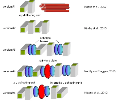
Several technologies have been developed to generate 3D readouts of fast population and dendritic activities, including liquid lenses (Grewe et al., 2011), deformable mirrors, temporal and spatial multiplexing (Durst et al., 2006; Cheng et al., 2011), axicon or planar illumination-based imaging (Holekamp et al., 2008), fast z-scanning based on an axially moving mirror (Botcherby et al., 2012), holographic scanning (Nikolenko et al., 2008), piezo- scanning with sinusoidal and non-linear resonance (Gobel et al., 2007; Katona et al., 2011), simultaneous multiview light-sheet microscopy (Tomer et al., 2012), and optical fiber acousto-optical (AO) deflector based 3D scanning (Rozsa et al., 2007). AO scanning technology has also been used to rapidly change beam focusing without mechanical movement (Kaplan et al., 2001), and AO technology for two-photon microscopy has been adapted in several applications (Kaplan et al., 2001; Reddy and Saggau, 2005; Iyer et al., 2006; Salome et al., 2006; Rozsa et al., 2007; Vucinic and Sejnowski, 2007; Duemani Reddy et al., 2008; Otsu et al., 2008; Grewe and Helmchen, 2009; Grewe et al., 2010; Kirkby et al., 2010).

However, in 2012 there were limitations in the use of these methods for 3D optical recordings both in vitro and in vivo. In in vitro applications, new 3D technologies either were

(38)

not validated in functional measurements on biological samples (Kaplan et al., 2001; Reddy and Saggau, 2005; Durst et al., 2006; Rozsa et al., 2007; Kirkby et al., 2010) or they did not simultaneously fulfill a set of technical criteria which are necessary to follow propagation of APs or Ca²⁺ spikes in dendrites over hundreds of micrometers.

Namely,

 less than 30 µm z-scanning were shown (Kaplan et al., 2001; Reddy and Saggau, 2005; Iyer et al., 2006; Salome et al., 2006; Rozsa et al., 2007; Vucinic and Sejnowski, 2007; Duemani Reddy et al., 2008; Holekamp et al., 2008; Nikolenko et al., 2008;

Otsu et al., 2008; Grewe and Helmchen, 2009; Grewe et al., 2010; Kirkby et al., 2010;

Katona et al., 2011),

 less than 20 measurement points were shown (Kaplan et al., 2001; Stosiek et al., 2003; Reddy and Saggau, 2005; Durst et al., 2006; Salome et al., 2006; Rozsa et al., 2007; Vucinic and Sejnowski, 2007; Duemani Reddy et al., 2008; Nikolenko et al., 2008; Grewe and Helmchen, 2009; Kirkby et al., 2010; Grewe et al., 2011; Botcherby et al., 2012),

 or less than 100 Hz repetition rate were demonstrated (Durst et al., 2006; Salome et al., 2006; Gobel et al., 2007; Rozsa et al., 2007; Nikolenko et al., 2008; Cheng et al., 2011; Grewe et al., 2011; Tomer et al., 2012) in these previous studies.

Regarding in vivo applications, random-access recording of the activity of hundreds of selected neurons situating in 3D was not validated until 2012. After we had published our 3D microscope (Katona et al., 2012) two other groups also published biological results with the use of 3D AO microscopes, however their 3D scanning volume is still an order of magnitude smaller than our scanning volume and they have shown less number of cells recorded simultaneously and smaller depth penetration (Cotton et al., 2013; Fernandez- Alfonso et al., 2014).

As mentioned in chapter 2.2, AO scanning as single-point two-photon ROI scanning approach can significantly increase the SNR of the signal measured from a ROI in a unit time, as compared to classical raster scanning. Quantitatively, by modifying Equation 3 to the 3D case yields:

(39)

Equation 4.

In a typical in vivo measurement, when we consider using a 450 x 450 x 650 µm³scanning volume (Katona et al., 2012) and measure 100 neurons of diameter of 10 µm, random access scanning will provide a 50 fold gain in the SNR.

4.2 Principles

The phrase “acousto-optic” refers to the field of optics that studies the interaction between sound and light waves. The sound generated pressure fluctuations cause a periodic change in the refractive index of the medium (usually tellurium dioxide) which behaves like an optical grating: diffracting light according to its period length and the wavelength of the light.

4.2.1 Acousto-optical deflection

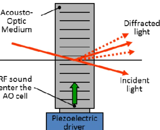
AO deflectors control the direction of the optical beams by ultrasonic waves. During operation, ultrasonic waves induced via a piezoelectric transducer diffract the laser beam depending on the driving frequency of the transducer (Kaplan et al., 2001). The change of the diffraction angle is given by

Equation 5.

where λ is the optical wavelength of the beam, ν is the velocity of the acoustic wave, and Δf is the change of the sound frequency (Figure 7). Diffracted beam amplitude depends on a number of geometrical parameters and the acoustic energy (Veress et al., 2010). The device is ideal for random-access beam positioning as the frequency of the driving voltage can be changed quickly, thus beam steering is not limited by mechanical inertia of any moving parts.