Development of 3D two-photon acousto-optical measurement methods for neuroscience studies
PhD thesis
Szalay Gergely
Semmelweis University
Szentágothai János Doctoral School
Supervisor: Dr. Rózsa Balázs, M.D., Ph.D.
Official reviewers: Dr. Szabadics János, Ph.D.
Dr. Kis Petik Katalin, Ph.D.
Head of the Final Ex. Committee: Dr. Kellermayer Miklós, M.D., DSc Members of the Final Ex. Committee: Dr. Tretter László, M.D., DSc
Dr. Ulbert István, M.D., DSc
Budapest
2018
1 C
ONTENT1 CONTENT ... 2
2 ABBREVIATIONS ... 5
3 INTRODUCTION ... 6
3.1 WHY DO WE NEED TO MEASURE NEURONAL ACTIVITY IN 3D? ... 6
3.1.1 Detecting activity with light ... 6
3.1.2 Two-photon excitation ... 7
3.2 3D ACOUSTO-OPTICAL MICROSCOPY ... 10
3.2.1 Acousto-optical deflection ... 10
3.2.2 Acousto-optical focusing ... 11
3.2.3 3D scanning configurations ... 11
3.2.4 The 3D-AO microscope ... 13
3.3 NOVEL GENETIC TOOLS FOR DETECTING CA2+ IN NEURONS ... 14
3.3.1 GCaMP6 sensor ... 14
3.3.2 Increased imaging depth with GCaMP6 ... 15
3.4 RADOM-ACCESS 3D ACOUSTO-OPTICAL SCANNING ... 17
3.4.1 In vivo demonstration of 3D imaging ... 19
3.4.2 Movement artifacts ... 20
4 AIMS ... 22
5 METHODS ... 25
5.1.1 Mice ... 25
5.1.2 Slice preparation and electrophysiology ... 25
5.1.3 Intrinsic imaging ... 26
5.1.4 AAV vector injection. ... 27
5.1.5 Surgical procedure ... 27
5.1.6 Visual stimulation ... 28
5.1.7 Virtual reality environment ... 29
5.1.8 In vivo electrophysiology ... 30
5.1.9 Data processing ... 30
6 RESULTS ... 31
6.1 THE NEW AO SCANNING SYSTEM ... 31
6.2 DISPERSION COMPENSATION ... 36
6.2.1 Material dispersion compensation ... 36
6.2.2 Calculating material dispersion introduced by the optical pathway ... 37
6.2.3 Determining prism compressor axis lengths ... 39
6.2.4 Angular dispersion compensation. ... 43
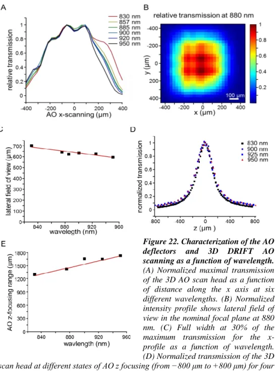
6.3 INCREASED TRANSMITTANCE EFFICACY AND SCANNING VOLUME AT LONG WAVELENGTHS ... 46
6.4 CONTINUOUS 3DTRAJECTORY SCANNING WITH AO DEFLECTORS ... 51
6.4.1 Moving the focal spot in 2D ... 53
6.4.2 Moving the focal spot in 3D ... 56
6.4.3 Fast 3D DRIFT AO microscopy ... 59
6.5 CORRECTION FOR THE MOTION INSTABILITIES ... 64
6.5.1 Beam stabilization ... 64
6.5.2 Automatic drift compensation algorithm ... 65
6.5.3 Offline motion correction using AO DRIFT scanning... 68
6.6 SCANNING METHODS FOR MOTION CORRECTION ... 69
6.6.1 3D ribbon scanning to compensate in vivo motion artifacts ... 69
6.6.2 Recording of spiny dendritic segments with multiple 3D ribbon scanning 70 6.6.3 Multi-layer, multi-frame imaging of neuronal networks: chessboard scanning ... 74
6.6.4 Multi-layer, multi-frame imaging of long neuronal processes ... 75
6.6.5 Volume scanning with snake scanning and multi-cube ... 78
6.6.6 Multi-3D line scanning ... 81
6.6.7 Advantage of the different scanning modes ... 82
6.6.8 Motion correction in 3D ... 83
6.6.9 Simulation of the quality increment with drift scanning ... 86
6.6.10 Validation of the fast 3D motion-detection method and recording brain movement ... 91
6.6.11 Single action potential measurement ... 94
6.7 RANDOM EQUIVALENT-TIME SAMPLING, SELECTION OF THE FLUORESCENT DYE . 98 6.7.1 Spatial distance estimate corresponding to the highest temporal resolution in bAP measurements. ... 101
6.7.2 Theoretical calculation of the maximal temporal resolution. ... 103
7 CONCLUSION ... 106
7.1 BENEFITS OF THE NEW 3D METHODS IN NEUROSCIENCE ... 107
7.2 IMAGING BRAIN ACTIVITY DURING MOTION ... 108
7.3 COMPENSATION OF MOVEMENT OF THE BRAIN ... 109
7.4 SIMULTANEOUS 3D IMAGING OF APICAL AND BASAL DENDRITIC ARBOR ... 110
7.5 DEEP IMAGING ... 110
CREDIT ASSIGNMENT ... 112
8 SUMMARY ... 113
9 ÖSZEFOGLALÁS ... 114
10 REFERENCES ... 115
11 REFERENCES BY THE AUTHOR ... 119
11.1.1 Publications connected to the Thesis ... 119
11.1.2 Other publications ... 119
12 ACKNOWLEDGEMENT ... 121
2 A
BBREVIATIONS3D – three dimensions
AAV – adeno-associated virus ACSF – artificial cerebral fluid AO – acousto-optics
AOD – acousto-optical deflector AOM – acousto-optical modulator AP – action potential
bAP – backpropagation action potential CA1 - Region I of hippocampus proper CW – continuous wave
EPSP – excitatory postsynaptic potential FWHM – full with at half maximum
GCaMP - the fusion protein containing the calmodulin-binding domain from the myosin light chain kinase also called M13 peptide, the circularly permutated green fluorescent protein, and the calmodulin
GECI – genetically encoded calcium indicator GDD – group delay dispersion
GFP – Green Fluorescent Protein IPSP – inhibitory postsynaptic potential LOTOS – low-power temporal oversampling MRT - magnetic resonance tomography NA – numerical aperture
OGB-1 – Oregon Green Bapta-1
OGR - Orvosi Géntechnológiai Részleg (KOKI) PET - positron emission tomography
PMT – photomultiplier tube PSF – point spread function RF – radio frequency ROI – region of interest SD – standard deviation SEM – standard error of mean SNR – signal to noise ratio TeO2 – tellur-dioxide
TOD – third order dispersion V1 – visual cortex 1
VR – virtual reality
VIP – vasoactive intestinal protein
3 I
NTRODUCTION3.1 Why do we need to measure neuronal activity in 3D?
To better understand neuronal computation fast readout of information flow and processing is essential since action potentials, dendritic integration, subthreshold EPSP and IPSP events all happen at the millisecond timescale. Moreover, neuronal diversity, layer specificity of information processing, area-wise specialization of neuronal mechanism, internally generated patterns, and dynamic network properties all suggest that fast recording is required not only from a single plane or point, but also at a level of large neuronal populations situated in large 3D volume1,2,3. In addition, coding and computation within neuronal networks are generated not only by the somatic integration domains, but also by highly non-linear dendritic integration centers, which in most cases remain hidden from somatic recordings4,5,6,7. Therefore, to get better insight in the details of these functions we need to simultaneously read out neural activity both at the population and single-cell levels, with sufficient spatial (in the µm range) and temporal (at the millisecond scale) resolution.
3.1.1 Detecting activity with light
Light microscopy has an important role in biological research since it unfolds the possibility to simultaneously investigate neuronal activity and morphology from living tissue with high spatial resolution, resolving not only cells and cells’ firing rate, but also subcellular compartment and subthreshold activity. However, the optical resolution is limited by the wavelength of the emitted light (according to Abbe’s rule) and does not rival that of electron microscopy, but the scope of electron microscopy is limited when observing living specimens8. Other vital imaging technologies, such as MRT (magnetic resonance tomography), PET (positron emission tomography) or X-rays, can neither resolve subcellular structures nor can provide the exquisite molecular selectivity that would allow single molecules to be detected with billions of others in the background9,10.
During the past decade several new optical methods have been developed for fast readout of neuronal network activity in 3D. For example, it is possible to record 3D structures using spatial light modulators11, liquid lenses12, acousto-optial (AO)
deflectors13,2,14, temporal multiplexing15, axicon or planar illumination-based imaging16, fast z-scanning based on an axially moving mirror17, piezo actuators2,18, simultaneous multi-view light sheet microscopy19, two-photon light sheet microscopy20, optical fibers addressed by AO deflectors21, light field microscopy22, phase-locked ultrasound lens23, or phase mask combined with holographic illumination24.
Light microscopy inside living tissues is hampered by the degradation of resolution and contrast, caused by absorption and light scattering, which appear in a varying degree in every tissue, due to refractive index inhomogeneity. The deeper we image in the tissue, images become more degraded and high-resolution imaging eventually becomes impossible. A major step towards overcoming this problem was the invention of confocal microscopy25,26. In a confocal microscope, the illumination light is focused on a diffraction-limited spot, and this excites the sample along two cones close to the aimed focal point. Then, using the same objective, the emitted signal photons are focused onto a detector pinhole that rejects all light emitted outside of the focus spot.
3.1.2 Two-photon excitation
The main drawback of confocal microscopy is its wasteful use of both excitation and emission. On one hand, absorption occurs throughout the specimen, but information is obtained only from a small sub-volume around the focal point. On the other hand, light that is scattered by the tissue, even if it is emitted from the focal point, is also rejected by the pinhole: this means that tissue scattering has a significant impact on the signal-to- noise ratio (SNR) of the images. This is particularly a major problem for in vivo fluorescence microscopy, where the limiting factors are usually either photochemical destruction of the fluorophore (photobleaching) or photodynamic damage to the specimen (photodamage)35. In confocal microscopy, only ballistic photons that are not scattered on their path out of the tissue contribute to the signal, while scattered photons, often the majority, are rejected by the detector aperture, limiting depth penetration of the technology to about 50-80 µm in brain tissue. Excitation needs to be increased in order to compensate for this signal loss, which further intensifies photobleaching and photodamage35. These problems are common to many other, so-called single photon excitation technologies, among them the spinning-disc confocal27 and light sheet
microscope technologies19. Theoretically, these problems can be handled by the use of laser scanning microscopy in combination with two-photon excitation19,28.
The concept of two-photon excitation is based on the idea that two photons of low energy can be combined in the same quantum event, resulting in the emission of a fluorescence photon at a higher energy than either one of the two excitatory photons.
The probability of such absorption is extremely low, its cross section is proportional to the square of the photon flux, making it possible to counterbalance this low initial cross section by using extremely high photon fluxes. Multi-photon absorption is often called nonlinear because the absorption rate is dependent on a higher-than-first-power light intensity. Such high fluxes are only present in the focus of a high numerical aperture lens illuminated by a strong, pulsed near-infrared laser. The possibility of absorbing more than one photon during a single quantum event had been predicted more than 80 years ago by Maria Goeppert-Mayer29, but it was confirmed experimentally only after the invention of mode-locked lasers with a pulse duration below 1 ps and repetition rates of about 100 MHz. This made two-photon laser scanning microscopy feasible in practice30.
Mode-locking a Ti:sapphire laser, for example, boosts the two-photon excitation rate by 100,000-fold, compared to continuous-wave (CW) laser operation with the same average power (since its light pulses or packages present only in the 100,000th part of the whole imaging time). This quadratic dependence of the absorption rate on the light intensity gives two-photon microscopy its optical sectioning property because fluorescence is only generated in the vicinity of the geometrical focus where the light intensity is high. While scanning the laser focus in both lateral directions (x and y), fluorescence excitation is limited to the focal plane. No detector pinhole is necessary since – in most cases – no fluorescence is generated outside the focal volume, and all fluorescence photons, whether leaving the sample on scattered or ballistic trajectories, constitute useful signal.
The combination of low phototoxicity is enabled by the single point excitation and the efficient use of fluorescence – even scattered photons can be detected – which makes single-point two-photon microscopy a unique tool for observing function deep within tissue, even resolving structures deeper than one millimeter in brain tissue31,32,33. Its main drawback, however, its lower acquisition speed when compared to camera-based
approaches where, instead of the ‘single-channel’, or single point photomultipliers (PMTs), information can potentially be collected from millions of camera pixels simultaneously.
From the technologies listed above only a handful can provide single-point multi- photon excitation in three dimensions that allows whole-field detection of the scattered fluorescence photons required for deep brain imaging31. Furthermore, among the available 3D scanning solutions for multi-photon microscopy, only 3D AO scanning is capable of performing 3D random-access point scanning2,14,34 to increase the measurement speed and signal collection efficiency by several orders of magnitude in comparison to classical raster scanning. This is because the pre-selected regions of interest (ROIs) can be precisely and rapidly targeted without wasting measurement time on unnecessary background areas whereas 3D AO technology enables freely “jump” the focus of the laser between these ROIs within microseconds.
3.2 3D acousto-optical microscopy
The 3D acousto-optical (3D-AO) microscopes, presented in the literature, possess different optical design and different performance, with their advantages and limitations. However, every design is based on the same physical principles, on the acousto-optical effect generated in reciprocate crystal.
The phrase “acousto-optic” refers to the field of optics that studies the interaction between sound and light waves. In the field of fluorescent imaging we use acousto- optical devices to diffract laser beams through ultrasonic gratings. The acousto-optical effect is based on a periodic change of the refractive index in a high refractive index medium (usually tellurium dioxide, Te02) which is the result of the sound wave induced pressure fluctuation in the crystal. This grating diffracts the light beam just like a normal optical grating, but here the gradient can be rapidly adjusted by changing the driving signal.35
3.2.1 Acousto-optical deflection
Acousto-optical deflectors (AODs) control the optical beam spatially, they use ultrasonic waves to diffract the laser beam depending on the acoustic frequency. If we introduce a sine wave at the piezoelectric driver, it will generate an optical deflection in the acousto-optic medium according to the following equation:35
𝛥𝛩
𝑑=
𝜆𝜈𝛥𝑓
(Equation 1)where λ is the wavelength of the optical beam, ν is the velocity of the acoustic wave, and Δf is the change in the sound frequency (Figure 1).
In practice, AODs or acousto-optical modulators (AOMs) are used. AOMs modulate only the amplitude of the sound waves, while AODs are able to adjust both the amplitude and frequency.
Figure 1. Operating principle of acousto-optical deflectors. A piezoelectric driver elicits radio frequency (RF) sound waves due to the externally applied sinusoidal voltage. Sound enters and traverses through the diffracting (TeO2) medium while interacting with light throughout the aperture. Light is diffracted on the sound wave’s refraction index changes as on a steady optical grating providing diffracted light beams whose angle is dependent on the sound wave’s frequency.
3.2.2 Acousto-optical focusing
Besides deflection, AODs can also be used for fast focal plane shifting2,14,34,36. If the frequency of the acoustic wave that fills up the crystal is changing linearly in time, (thus the frequency is chirp), then at a given point in the crystal the optical gradient increases as a function of time, so different portions of the optical beam are deflected in different directions (Figure 2). Thus focusing or defocusing effect occurs, depending on the frequency slope (sweep rate) of the chirped acoustic wave. The focal length of an acousto-optical lens (F) can be calculated from the sweep rate as36:
𝐹 =
𝜈2𝑇𝑠𝑐𝑎𝑛2𝜆𝛥𝑓 (Equation 2)
where λ is the optical wavelength of the beam, ν is the velocity of the acoustic wave, Δf is the change of the sound frequency, and Tscan is the modulation rate of the sound frequency36.
To keep a stable focal distance, the frequency gradient should be preserved in the crystal. The frequency should therefore be continuously increased (or decreased) at the piezoelectric driver to preserve the focal distance. This will result in a lateral drift of the focal-point, which can be easily compensated by introducing a second acousto-optical deflector with a counter-propagating acousto-optical wave into the optical pathway36.
Figure 2. Acousto-optical focusing. AO deflector arrangement similar to Figure 1, but here the sound frequency is changing, resulting in a varying grating size along the propagation axis. As a consequence, different parts of the laser beam are diffracted with varying angles creating a focus point whose position can be changed by the parameters of the sound applied to the deflector. Red and yellow lines indicate diffracted and incident laser beams and F denotes focal distance.
3.2.3 3D scanning configurations
Combining four of these crystals can form a 3D focusing system. We need two orthogonal deflectors for X and Y scanning, a third one for Z focusing, and we need a
forth one to compensate for the drift caused by the Z focusing crystal. The four deflectors can be organized to a focusing system at several configurations (Figure 3).
We have designed the detailed optical model of these configurations to find the combinations of active and passive optical elements in the scanning light-path of the microscope, which would provide the maximal exploitation of the apertures of all lenses at different X, Y and Z scanning positions, and therefore result in the smallest PSF in the largest possible scanning range.
The model suggested a new design concept. The largest scanning volume can be reached by grouping the deflectors into two functionally distinct groups which are coupled by one afocal projection (Figure 4).
Figure 3. Different 3D AO scanning arrangements. Version #1 uses optical fibers to position the excitation beam in 3D21, however it has been difficult to implement this version due to the requirement of many mechanical devices positioning the fibers. Versions #2-5 were analyzed by modeling and Version #5 was found the most beneficial to implement2. Version #214,37 and Version #413,34,38,39
have been described by other laboratories and have recently been used for functional measurements13,34 but – according to our expectation from optical modeling – they have lower specifications than our solution.
3.2.4 The 3D-AO microscope
Figure 4 shows the schematic of the earlier version of the 3D-AO microscope used in our lab (see more details in Katona et al. 2012). Briefly, laser pulses were provided by a femtosecond laser source. The beam was extended to 15 mm by a Galilean telescope in order to fill the large aperture of the acousto-optical deflectors. Z-focusing and lateral scanning were achieved by two separate pairs of acousto-optical deflectors which were coupled by two achromatic lenses (f = 200 mm). Finally, the light was coupled to an upright two-photon microscope (Femto2D, Femtonics Ltd.) using a telecentric relay consisting of an f = 250 mm and a f = 210 mm lens (Thorlabs). The excitation was delivered to the sample, and the fluorescent signal was collected, using an Olympus 20×, NA 1.0 objective and then separated using a dichroic mirror (700dcxru, Chroma Technology). The separated fluorescence was delivered to GaAsP photomultipliers fixed on the objective arm, short focal distance lenses were used the focus to light to the detectors surface. During in vitro measurements the fluorescence photons propagating opposite to the objective were also captured by similar photomultipliers mounted below the condenser lens in order to enhance the collection efficiency of the scattered photons.
Figure 4. Simplified optical path of the 3D-AO microscope – The first pair of acousto-optical crystals were used for X,Y scanning while the second pair for Z-focusing. Angular dispersion was compensated for better optical resolution through the whole field of view. Described in more detail in Katona et al. 2012; Szalay et al. 2016.
3.3 Novel genetic tools for detecting Ca
2+in neurons
3.3.1 GCaMP6 sensor
Besides a fast and reliable scanning method the other pillar of functional anatomy is an adequate labeling technique which makes biological activity visible for fluorescent microscopy. Regenerative neuronal events are coupled with the flux of several ions, including sodium, potassium, calcium and in some cases chloride or other ions.
However the absolute concentration is larger for sodium or potassium the relative change is much larger, in the order of magnitude, for calcium. Therefore in the literature activity sensitive dyes, almost exclusively, are designed to be coupled with calcium concentration change. That is why intracellular calcium indicators will indicate activity, and calcium concentration increase with increase of excitable molecule. This change can be followed for example with two-photon microscopy, but also with other techniques.
Fluorescent calcium sensors can be synthetic dyes or protein based molecules. Using structure-based mutagenesis and neuron-based screening a new family of ultrasensitive protein calcium sensors (GCaMP6) was developed that outperformed other sensors in cultured neurons, zebrafish, flies and also in mice in vivo40. With GCaMP6 sensor, under ideal circumstances, even detection of single action potentials in neuronal somata or in individual dendritic segments15 is feasible from layer 2/3 pyramidal neurons of the mouse visual cortex. Thus this sensor provides new insight into the organization and dynamics of neural circuits over multiple spatial and temporal scales40.
According to Chen et. al 2013, supported by our own experience (Figure 5), the GCaMP sensor have maintained signal levels compared to bulk loaded AM dies. Beside this maintained signal level, GCaMP6 labeling has several other advantages:
(i) Labeling is more stable over long timescales. Since uptake and clearance of synthetic dies occur on a much faster time scale, over hours, baseline fluorescence level can change over a long measurement day. Therefore, it is impossible to perform several days or weeks long measurements with this die, while viral labeling can be stable even for months, without no or modest change in the baseline florescence level41. This allows longer experimental
protocols, raising the possibility to combine this measurement with behavioral protocols.
(ii) With the combination of different promoters, it allows simultaneous measurement of spines and somata from several cells40.
(iii) Most importantly, since it is a genetic method we can selectively label different cell types.
(iv) Allows deeper imaging from the tissue.
Figure 5. Calcium responses from GCaMP6f labeled animals. Ca2+ responses are measured form whole cell patch clamed CA1 pyramidal cell in vitro. Cells were labeled with GCaMP6f with AAV viral injections. bAPs were induced by voltage injections through the patch pipette.
Fluorescent signal measured on the somata or on a 50-100 µm segment of the apical dendrite.
(Right) Measured fluorescent transients for 1, 2, 3, 4, 5, 8, 10 and 14 action potentials shown as ΔF over F. (Middle) Average maximums from the transients in the Left. (Right) Representative electrophysiology data, shown for 1, 2, 5 and 10 action potentials. For all measurements AP frequency was 20Hz.
3.3.2 Increased imaging depth with GCaMP6
Deep imaging within the tissue can help us to measure larger portion of the neuronal network under investigation. The increased scanning depth is resulted by the fact that this genetically encoded calcium indicator can be emitted at longer wavelength compared to the previously used most popular synthetic dyes (850-960 nm for GCaMP family compared to 780-850 nm for synthetic dies such as OGB-1, Fluo-4 or Fluo-5F).
This difference enables measuring deeper from the tissue, as imaging depth during two-
photon measurements determined is mainly by the emission spectra. This is the result of the absorption properties of living tissue, since during two-photon imaging excitation wavelength falls to the near infrared range, where biological tissue is mostly transparent; however, emission spectra falls in the visible range, thus much more influenced by re-absorption, diffusion and scattering caused by the tissue.
Figure 6 shows the wavelength dependent imaging depth where I pulled data from all measurement I performed in vivo during this work. Imaging depth was defined as the Z- range of the imaging point during the experiment. Obviously, this representation does not take several parameters into account, such as surgery quality, cranial window size, number of blood vessels in the imaging field, optical resolution, die concentration, which can all influence imaging depth during two-photon imaging. Still the tendency shown on Figure 6 supports the idea that by developing dies with longer wavelength can help image deeper in the tissue. This idea is also demonstrated by three-photon imaging where the emission wavelength is even longer (in the 1500 nm range) and can reach imaging depth of 1200 µm42.
Figure 6. Wavelength dependent imaging depth. Data is pulled from all in vivo measurements I have performed during the work for this thesis. Each data point indicates a single measurement. The imaging depth indicated the Z-range of measurement points during the given experiment. I only include those measurements where the imaging data was used for the analysis of a given biological project, thus the one which are “good enough” for biological measurement, to minimize the effect of the surgery, bone regrown or other non-correlated parameters. Light green points show OGB-AM, dark green GCaMP6f, light red RCaMP1 while dark red jRGECO measurements.
3.4 Radom-access 3D acousto-optical scanning
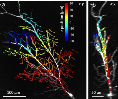
To demonstrate imaging performance of 3D point scanning I have imaged backpropagating action potential (bAP) at several dendritic sites. I patch-clamped a CA1 pyramidal cells in whole-cell mode in an acute hippocampal mouse brain slices and filled the cells with the green fluorescent Ca2+ sensor Fluo-5F and the red fluorescent marker Alexa594. On the example presented on Figure 7 propagating activity was measured at seventy-seven 3D locations of a single hippocampal neuron.
The objective was positioned at a depth such that the center of the region of interest was in focus. The objective was fixed at this position and a reference z-stack of images was acquired using 3D AO scanning only(Figure 7), then measurement points were selected along the dendritic tree. The cell was held in current-clamp mode and an AP was evoked by somatic current injection while near-simultaneously measuring dendritic Ca2+ signals associated with the bAPs by repetitively scanning the selected 3D coordinates with 29.76 kHz. When sample drift occurred, I’ve repositioned single points or the entire group manually.
Figure 7. Three-dimensional measurement of bAPs. (a) Maximum intensity z-projection of the dendritic arbor of a CA1 pyramidal cell imaged with 3D AO scanning. Circles represent the 77 pre-selected measurement locations for 3D random access point scanning. Overlaid curves show Ca2+ transients recorded near-simultaneously in each location induced by a single bAP (each average of five traces). The repetition rate of the measurement was 29.76 kHz (0.39 kHz speed in each location). The z coordinates of the measurement locations are color-coded. (b) Maximum intensity side projection of the cell with the measurement locations shown in a.
Since the acute brain slices were 300 µm thick, only a fraction of the total AO z- scanning range was used. To test random-access 3D AO scanning for a larger z-range I have record bAP-induced Ca2+ transients while moved the objective focal plane mechanically from + 562 µm to − 546 µm away from the z-center and used AO z- focusing to refocus the recorded dendritic tree (Figure 8). Independent of the AO z- settings, single bAPs could be resolved in Ca2+ transients induced by a train of three APs. Similarly, single bAPs could be followed in a 760 µm lateral scanning range (Figure 8b). Thus a total of 1190 µm AO z-focusing range and a 760 µm AO lateral scanning range is shown with the 20× objective where single APs can be resolved with SNR over 2. In summary, resolution of single AP-induced transients is possible in a near-cubic-millimeter scanning volume during in vitro conditions.
Figure 8. Resolving bAPs at the sides of the FOV. (a) Single traces of three bAP-induced dendritic Ca2+ transients measured at the same dendritic point at different AO z-focusing settings. To keep the image sharp, the AO z-focusing was compensated by mechanical refocusing of the objective. Note the preserved single AP resolution even at the lower and upper limits of the scanning range. Corresponding somatic voltage traces (Vm) are shown on the top (b) The same as in c, but transients were recorded while shifting the dendrite along the x axis.
(c) The same as in a, but single traces were recorded using the 16× objective. Note that the AO z-focusing range with single AP detection level exceeds 2000 μm (for in vitro conditions and in transparent sample).
3.4.1 In vivo demonstration of 3D imaging
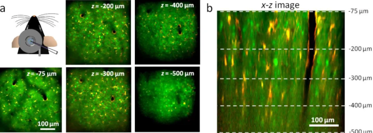
To demonstrate 3D imaging also at in vivo circumstances, I’ve recorded Ca2+ responses from a population of individual neurons in the visual cortex of adult anesthetized mice.
I’ve injected a mixture of OGB-1-AM to monitor changes in intracellular Ca2+
concentrations, and sulforhodamine-101 (SR-101)43, to selectively label glial cells (Figure 9). The red fluorescence of SR-101 allowed differentiation between neurons and glial cells (green and red). The maximal power of our laser (3.5 W at the laser output and ~180mW after the objective) limited the depth of the in vivo recording to a maximum of 500 µm from the surface of the cortex (the total imaging volume was 400×400×500 µm).
Figure 9. In vivo image stacks of the neuronal population. (a) Representative background- corrected images taken at different depths from the surface of the brain showing neurons (green) and glial cells (red and yellow). (upper left) Sketch of in vivo experimental arrangement. Staining by bolus loading (OGB-1-AM and SR-101) in mouse V1. (b) x-z slice taken from the middle of the stack volume Dotted lines correspond to the planes in a.
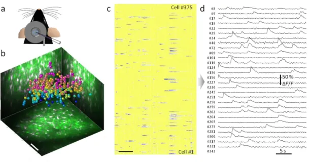
Next, we recorded a reference z-stack and, either by using an automated algorithm, or manually, we identified the neuron and glial cell bodies. In the simple case when OGB1-AM and SR-101 dyes are bolus loaded into the animal, cells can be categorized according to their dye content measured by fluorescence, which is possible on multiple channels. In this case neuronal cells can be detected from their elevated green fluorescence and decreased red fluorescence. Centers of each neuronal cell body were used for random-access activity imaging (Figure 10b).
After the selection of the cell bodies, we recorded the activity of each neuron by scanning at 80 Hz and plotted the recorded raw and point-by-point background-
corrected and normalized fluorescence data in real-time, each row showing the activity of a single cell (Figure 10c). Responses of neurons could be resolved with high SNR (Figure 10d). The stability of long-term recording was monitored using the baseline fluorescence.
Figure 10. Spontaneous neuronal network activity in vivo. (a) Sketch of in vivo experimental arrangement. (b) Maximal intensity side- and z-projection image of the entire z-stack (280×280×230 µm3; bolus loading with OGB-1-AM and SR-101). Spheres represent 375 autodetected neuronal locations color coded by depth. Scale bars, 50 µm. (c) Parallel 3D recording of spontaneous Ca2+ responses from the 375 locations. Rows, single cells measured in random-access scanning mode. Scale bar, 5 s. (d) Examples of Ca2+ transients showing active neurons in c.
3.4.2 Movement artifacts
Despite the evident benefits of the 3D point scanning, when we want to extend the scope of this scanning technique to behaving animal models, to measure a single point per neuronal structure will not be sufficient. Fluorescence information could be completely lost during motion in behaving animals when using the point scanning method (Figure 11).
To overcome this limitation we need to extend single scanning points to surface or volume elements in order to preserve the surrounding fluorescence information for motion artifact elimination.
The size of the surrounding area and temporal resolution of the measurement are working against each other, the proper extent is defined by the properties of the given
measurement. However measuring every point in the 3D volume needed for sufficient motion correction would increase temporal resolution to the second range, which not allows fast calcium measurement for burst or single action potential detection. This issue can be address by arbitrary 2D planes distributed in the 3D space, 3D AO technology is a great tool for the realization. The details of this method will be explained through this thesis.
Figure 11. Fluorescence information can be completely lost when using point-by-point scanning in the moving brain of behaving animals. Exemplified dendritic and spine transients were recorded using 3D random-access point scanning during motion (green) and rest (blue) from one dendritic and one spine ROI, indicated with white triangles in the inset. Note that fluorescence information can reach the background level in a running period, indicating that single points are not sufficient to monitor activity in behaving animals.
4 A
IMSDespite the evident benefits of 3D random-access AO microscopy, the method faces some limitations when we would like to perform long term measurements from awake, behaving animals, where long term stability and redundancy for motion artefact have key importance. The aim of my work was to outline and address these emerging problems and design novel techniques and measurement strategies which provide stable and reliable image quality for behavioral studies during everyday use.
These issues to handle are the following:
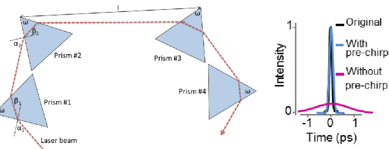
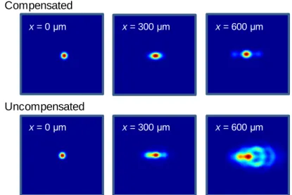
1) Dispersion compensation – Acousto-optical crystals are composed of high refractive index material thus introducing large material dispersion. Short light pulses (around 100 fs for Ti:Sa lasers) traveling in high refractive index material are elongated significantly, that reduces two-photon efficiency. In our system with 72 000 fs2 group delay dispersion (GDD) this effect would produce picosecond long pulses completely diminishing our two-photon signal during in vivo measurements. To compensate for this artifact, first we created the detailed optical model of the system containing all the optical elements and calculated the exact material dispersion produced by these components. Then we designed and built a four-prism compressor that fully aborts this error. Besides material dispersion AO crystals also introduce large angular dispersion caused by the spherical inhomogeneity of the AO crystals and other optical elements, which would produce position dependent elongation of the point spread function (PSF). At the edges of the imaging field the extent of this effect can be so large that, on one hand, resolution degrades so even somata cannot be resolved; on the other hand, laser intensity distributed in a larger focal volume would dramatically reduce quantum efficiency. To compensate for this, the exact properties of the angular dispersion were determined again from the optical model, and then fully compensated with a special lens introduced in the optical pathway.
2) Increasing transmittance at longer wavelengths – With the introduction of new genetic dies and sensors in neuroscience (for example GFP or genetically encoded calcium indicators, such as GCaMP6) the use of longer wavelengths became essential to effectively excite these molecules. Acousto-optical cells are highly
sensitive to the wavelength and this proportion is inverse. Since we are using four of these crystals in the optical pathway, the transmitted intensity drops dramatically when increasing wavelength. Changing the wavelength from 800 nm to 875 nm, without any additional compensation, would cause the transmittance to drop from 10% to around 1.5%, that is, even with the modern 2-3W femtosecond laser allowing only around 40mW imaging power, which is insufficient for in vivo measurement deep in the tissue. To overcome this limitation, we applied several optical and electronical developments in the microscope design, to achieve at least as high transmittance as previously with the shorter wavelength.
3) AO Drift scanning - Sampling rate is limited by the optical aperture of AO deflectors, which must be filled by an acoustic wave to address a given scanning point. In our system, with relatively large crystal length during 3D point-by-point scanning the switching time is relatively long (about 20-33 µs), which limits either the measurement speed or the number of ROIs. If we are measuring from a behaving animals, therefore have to measure multiple points per cell or dendritic segment, to produce data for motion correction, with random access point scanning mode the sampling rate would drop to the 1-2 Hz range, which is insufficient to resolve fast Ca2+ events.
To resolve this problem we introduce a new scanning method, 3D DRIFT scanning, which increase the scanning rate 3-70 fold depending on the measurement paradigm.
4) Motion artefact compensation - It has been shown that neuronal signaling could be completely different in awake and behaving animals44,45,46. Nevertheless fluorescence data are lost or contaminated with large amplitude movement artifacts during in vivo recordings in behaving animals, this occurs because the actual location of the recorded ROIs is continuously changing during the measurements due to tissue movement caused by heartbeats, blood flow in nearby vessels, respiration, and physical motion47. This results in fluorescence artifacts because of the spatial inhomogeneity in the baseline fluorescence signal and in relative fluorescence changes. In addition, the amplitudes of motion-induced transients can even be larger than the ones induced by one or a few action potentials detected by genetically encoded calcium indicators (GECIs)40.
Therefore it is difficult to separate post-hoc the genuine fluorescence changes associated with neural activity from the artifacts caused by brain movement. To overcome this problem we used 3D DRIFT AO scanning, extending the pre- selected individual scanning points to small 3D lines, surfaces, or volume elements to cover not only the pre-selected ROIs but also the neighboring background areas or volume elements while maintaining the data sampling rate.
Volume or area images acquired with the methods developed allow motion artifact correction on a fine spatial scale and, hence, the in vivo measurement of fine structures in behaving animals. In this way, we can preserve fluorescence information from the pre-selected ROIs during 3D measurements even in the brain of behaving animals, while maintaining the 20-400 Hz sampling rate that is necessary to resolve neural activity at the individual ROIs.
Another source of artifact caused by mechanical instability is the waggle of the beam itself caused by the instability of the optical elements. Reliable microscope stability in the daily routine is a very important factor. Since the optical path of the acousto-optical microscope is more than 6 meters long and containing more than a hundred optical elements, most of them sensitive of temperature and humidity fluctuation, active stabilization of the beam was necessary. This was realized with the combination of quadrant detectors and motorized mirrors.
5) Increased temporal resolution – If we are interested in even faster Ca2+ events, such as fine properties of sharpe-wave ripples, local regenerative events or signal propagation along a dendritic arbor, the 20-400 Hz sampling rate of 3D AO point scanning can be still insufficient. This limitation can be overcome at some circumstances, for example, when we have the event repeated many times with very precise timing. Given these circumstances we were able resolve sub millisecond or even microsecond events and measure the propagation speed even along a 10-20 µm segment of a dendritic branch.
5 M
ETHODS5.1.1 Mice
All experimental protocols were approved by the Animal Care and Experimentation Committee of the Institute of Experimental Medicine of the Hungarian Academy of Sciences (approval reference numbers PEI/001/194-4/2014 and PEI/001/1771-2/2015).
All procedures complied with Hungarian and European regulations for animal research, as well as with the guidelines of Society for Neuroscience. The in vivo recordings from the primary visual cortex were performed on C57BI/6J, Thy1-Cre, vip/IRES-Cre mice (P60-120). Animals were allowed free access to food and water and were maintained in temperature-, humidity-, and light-controlled conditions. Transgenic lines were developed and bred at the Medical Gene-technological Unit (OGR) of the Institute of Experimental Medicine of the Hungarian Academy of Sciences.
5.1.2 Slice preparation and electrophysiology
Acute hippocampal slices were prepared from Thy1-Cre mice (injected with Cre dependent version of GCaMP6f vector) using isoflurane anesthesia followed by swift decapitation, in accordance with the Hungarian Act of Animal Care and Experimentation (1998; XXVIII, section 243/1998.). Horizontal (300-400 μm) brain slices were cut with a vibratome and stored at room temperature in artificial cerebrospinal fluid (ACSF) (in mM: 126 NaCl, 2.5 KCl, 2 CaCl2, 2 MgCl2, 1.25 NaH2PO4, 26 NaHCO3, and 10 glucose) as previously described2,5,6.
Hippocampal CA1 pyramidal cells were visualized using 900 nm infrared lateral illumination5. Current-clamp recordings were made at 23°C or 33°C (MultiClamp 700B, Digidata 1440: Molecular Devices; chamber heater: Luigs & Neumann; in-line heater: Supertech). For whole-cell current-clamp recordings, glass electrodes (6-9 MΩ) were filled with (in mM): 125 K-gluconate, 20 KCl, 10 HEPES, 10 Di-Tris-salt phosphocreatine, 0.3 Na-GTP, 4 Mg-ATP, 10 NaCl. For fast-propagation speed measurements we added 0.2 mM Fluo-5F pentapotassium salt (Invitrogen) and 0.2 mM Alexa-594 (Invitrogen) to the pipette solution. For extracellular current-clamp recordings, glass electrodes (6-9 MΩ) were filled with ACSF or with ACSF containing 1 M NaCl. All chemicals and drugs, unless otherwise noted, were purchased from
Sigma. Cells with a resting membrane potential more negative than –50 mV were accepted.
Focal synaptic stimulation was performed as described earlier2,5,6. Briefly, 6-9 MΩ glass electrodes filled with ACSF were placed at a distance of 10-15 µm from the dendrite (stimulation: 0.1 ms, 10-50 V, 10 ms pulse interval, 1-3 stimuli; BioStim, Supertech).
Electrodes were targeted to the dendrite by a program written in MATLAB synchronizing the coordinate system of the patch-clamp manipulator and the microscope by the simultaneous use of two-photon imaging and transmitted oblique laser light data. Backpropagating APs were induced by somatic current injections (200- 400 pA, 5 ms; 1-3 bAPs were evoked at 50 Hz).
5.1.3 Intrinsic imaging
During in vivo imaging and viral injection, the V1 region was localized with intrinsic imaging. For recording intrinsic signal first the skin was opened and the skull over the right hemisphere of the cortex was cleared. The intrinsic signal was recorded using the same visual stimulation protocol we used later during the two-photon imaging session.
Figure 12. Intrinsic imaging. Left, absorption spectra of the oxy- and deoxy-hemoglobin shows that the highest relative difference in the absolute absorption of the two states of hemoglobin is present around 595nm, even if the highest absolute signal could have been detected with 550nm illumination. Right, normalized absorption of the brain surface 1-6s after the visual stimulation onset.
We could distinguish the region of interest by the absorption change in the given region, as described earlier48. Briefly, intrinsic imaging is based on the measurement of reflection change of the cortical surface. The source of the reflection change, depending
on the wavelength used for illumination, is either the change in oxygenization of the blood (595nm), or change in blood volume (550nm). Although the latter one has larger absolute signal, our aim was only to detect activation of V1, which could be detected more reliably with 595 nm illumination.
During the measurements we captured the baseline for 7 seconds in complete darkness, then moving bars were introduced for the mice for 7 seconds. Video signals were averaged for every second, and reflection change compared to baseline was calculated.
Protocol was repeated 32 times and signals were averaged.
5.1.4 AAV vector injection.
The injection procedure was adopted from Chen et al. 2011 and Wertz et al 2015 with some modifications. A 0.5 mm hole was opened in the skull with the tip of a dental drill over the V1 cortical region (centered on average 0.5 mm anterior and 2 mm lateral to the lambda structure – previously localized by intrinsic imaging). The glass micro- pipette (tip diameter ≈10 µm) used for the injections was back-filled with 0.5 µl vector solution (≈6×10¹³ particles/ml) then injected slowly (20 nl/s for first 50 nl, and 2 nl/s for the remaining quantity) into the cortex, at a depth of 450 µm under the pia. For population imaging we used AAV9.Syn.GCaMP6f.WPRE.SV40 or AAV9.Syn.Flex.GCaMP6f.WPRE.SV40 (in the case of Thy-1-Cre animals); both viruses were purchased from Penn Vector Core, Philadelphia, PA. For sparse labeling we injected the 1:1 mixture of AAV9.Syn.Flex.GCaMP6f.WPRE.SV40 and AAV1.hSyn.Cre.WPRE.hGH diluted 10,000 times. The cranial window was implanted over the injection site 2 weeks after the injection, as described in the surgical procedure section.
5.1.5 Surgical procedure
2-3 weeks after injection, mice were anaesthetized with a mixture of midazolam, fentanyl, and medetomidine (5 mg, 0.05 mg and 0.5 mg/kg body weight, respectively).
A circular craniotomy (3 mm diameter) was made above the V1 cortex (localized before virus injection with intrinsic imaging) without touching the dura mater.
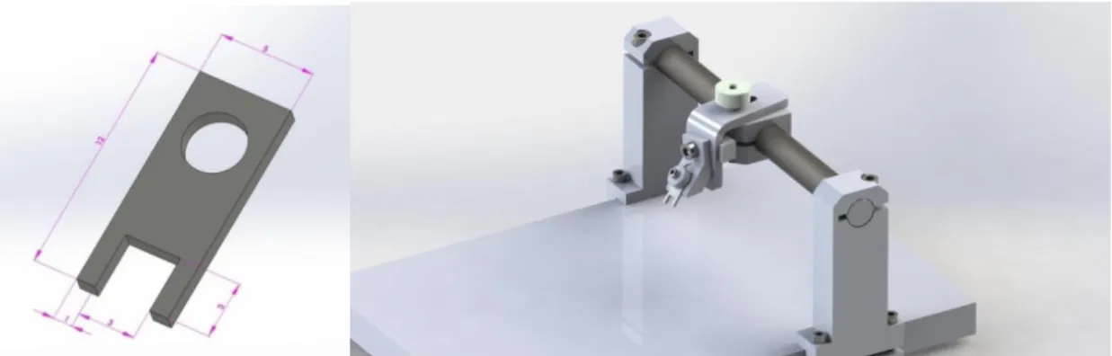
A custom-made aluminum head plate was fixed to the skull using cyanoarcylate glue and dental cement (Figure 13). During drilling, the place of craniotomy was rinsed
continuously with cold Ringer solution. When performing acute dendritic measurement the dura mater was also removed with a bended tip needle. The area of the craniotomy was covered with a double cover glass, as described previously49. For two-photon recordings, mice were awakened from the fentanyl anesthesia with a mixture of nexodal, revetor, and flumazenil (1.2 mg, 2.5 mg, and 2.5 mg/kg body weight, respectively) and kept under calm and temperature-controlled conditions for 10-20 minutes before the experiment. Before the imaging sessions, mice were kept head- restrained in the dark under the 3D microscope for at least 1 hour to accommodate to the setup. In some of the animals, a second or third imaging session was carried out after 24 or 48 hours.
Figure 13. Custom made mouse head holder used during the experiments. (Left) Headplate mounted to the mouse’s skull. (Right) In vivo holder.
5.1.6 Visual stimulation
A 15” computer monitor (Acer, 1280 x 768 pix resolution) placed 20 centimeters from the contralateral eye (covering ~100° × 70° of the visual field) was used to cast the visual stimuli generated by a program written in MATLAB using the ‘Psychtoolbox’
add-on package (http://psychtoolbox.org/wikka.php?wakka=HomePage). To prevent stray light from entering the objective, a black cover was placed over the complete visual stimulation path. Each trial of the visual stimulation started by showing a black screen with a non-moving grating appearing at the edge of the screen after 2 s; after 1 s, the grating moved in a direction orthogonal to its orientation for 5 s (drifting speed 1 cycle per 1 s), was stopped for 1s, and then disappeared, leaving a black screen for a further 1 s and between the trials. Trials with eight different grating directions were tested with an angular interval of 45°.
5.1.7 Virtual reality environment
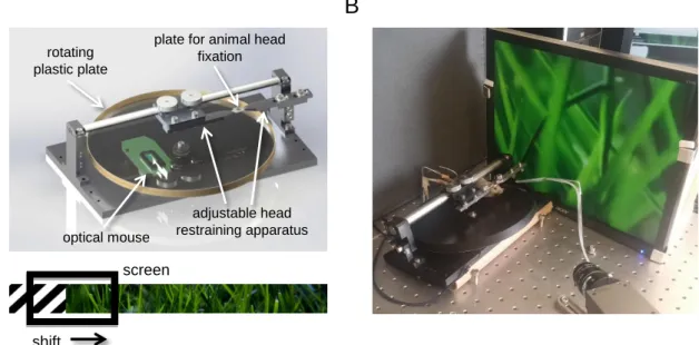
During the awake experiments, the mouse was head fixed, but free to run on a custom- designed linear treadmill made of a light rotating plastic plate (Figure 14). Easy rotation of the plate was provided by two ball-bearings (619/8, SKF). The motion of the treadmill was recorded with a high speed (1 kHz sampling rate) optical mouse (Urage reaper 3090, Hama) mounted upside down on the other side of the dial, and the angular displacement was recorded simultaneously at the same time as fluorescent signal. We used a self-developed script written in MATLAB to move the "wall" of the labyrinth on a 15” LCD screen according to the position signal of the optical mouse. Then we exported the output curves (velocity, position) to Excel for further analysis. Animals were habituated to the wheel for 20 minutes every day before the experiment, for at least three days, but no other behavioral training was used. For test of motion correction efficiency traces were divided into temporal intervals, running and rest, which were then separated by using a 2.6 mm/s speed threshold. See also Figure 14 for more details.
Figure 14. Virtual reality (VR). A linear treadmill was used to record the velocity of movement during fluorescent recording. (A) Solidworks image of the virtual reality environment. The position of a rotating light plastic plate was decoded by an optical mouse mounted upside down, and loaded into the MATLAB-based program. A 10 mm steel rod was stretched at both sides to minimize movement of the head-restraining apparatus during motion. A video screen placed in front of the left eye of the mouse was continuously updated according to the position signal with the actual part of an image. We realized a linear maze by teleporting the animal to the beginning of the VR image when it reached the end. (B) Image of the VR used with the 3D DRIFT AO microscope.
rotating plastic plate
B
optical mouse
plate for animal head fixation
adjustable head restraining apparatus
screen
shift
A
5.1.8 In vivo electrophysiology
To determine the correlation between Ca2+ transient and AP number, we performed cell- attached patch-clamp recording in in vivo conditions. The surgery was as described above, except for a small area left uncovered, about 1 mm wide, next to the cover glasses: this region was used as insertion site for the pipette, while the cells were measured under the cover glass, to limit tissue motion. For the recordings we used 7-8 MΩ-resistance borosilicate glass electrodes filled with extracellular solution, containing (in mM): 126 NaCl, 2.5 KCl, 2 CaCl2, 2 MgCl2, 1.25 NaH2PO2, and 100 µM Alexa 594 (Invitrogen) to visualize the pipette. Electrophysiological data were recorded in current- clamp mode with 0 mV holding potential simultaneously with the calcium imaging.
Transients were band-pass filtered between 1 Hz and 5 kHz and the number of APs was counted manually.
5.1.9 Data processing
Most of the analysis, including video rearrangement, motion correction, running average and ΔF/F calculation was performed with the built-in analysis tools in the acquisition software (MES, Femtonics Ltd., Budapest, Hungary). Raw fluorescence data (F) recorded along surface elements in 3D were spatially normalized, and then projected onto a 2D plot by applying the formula: ΔF/F = (F(dL,dtr1,t) – F0(dL,dtr1))/F0(dL,dtr1), where t denotes time, and dL and dtr1 indicate the longitudinal and the transversal distance along the ribbon, respectively. For 3D projection, 3D rendering, and 3D hyperstack analysis we used the ImageJ open-source software with some custom-written macros.
6 R
ESULTSFor reaching the settled aims, detailed in the previous section, we had to improve, on one hand, the imaging system for more reliable performance, and, on other hand, I had to design new measurement methodology for the most reliable use of these technical advances.
In the first part of the result section I will explain the technical advances that ensure the long-term reliable use of AO scanning from behaving animals. We made the following improvement compared to the previous system: (i) I have installed a four prism compressor and an angular drift compensation lens to the system, (ii) We designed new driving signals to the AO deflectors for faster scanning, (iii) and we designed new software component to realize new scanning methods.
6.1 The new AO scanning system
Before the detailed description of these developments, for the better understanding, I first explain the complete optical design of the final system, and then detail the necessity and function of the specific components. Since having an overall picture of the optical design will help to me to explain more easily the new developments in detail.
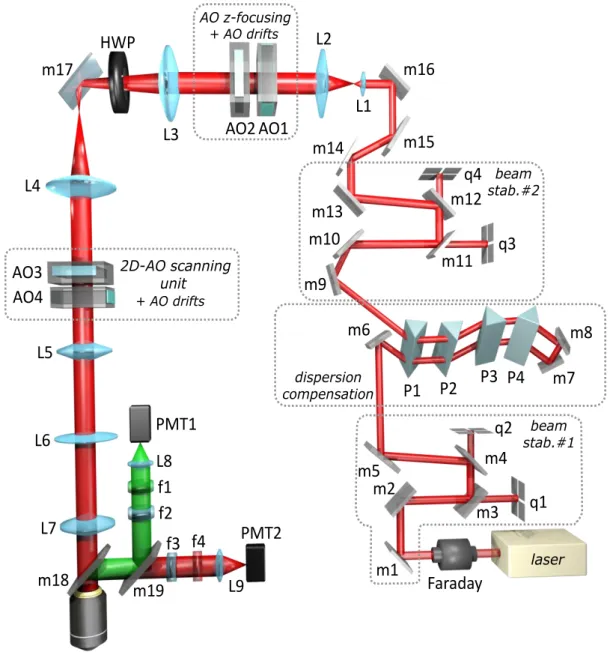
The 105 fs long laser pulses were delivered by a Ti:S laser at a 80 MHz repetition rate (Mai Tai, Spectra Physics, Figure 15). The coherent backreflections from optical elements were blocked by a new type of Faraday isolator (BB9-5I, EOT) that had a higher center wavelength (900 nm) and provided 5-10% higher throughput in the desired (850-950 nm) wavelength range (92% transmission at 900 nm) than the previous version2. The elimination of thermal drift errors were realized by two automated beam stabilization units (beam stab. #1 and #2). Each stabilization unit was built from two position sensors (quadrant detectors, q1-q2, and q3-q4) and two motorized mirrors (m1- m2, and m9-m10), wired in a feedback loop. The first beam stabilization unit contained the following items: m1, m2, m3, m4, m5, q1, and q2 (Figure 15), where m1 and m2 are silver mirrors (PF03-03-P01, Thorlabs) in piezoelectric mounts (ASM003, Thorlabs) controlled by a high voltage electronic controller (TPZ001, Thorlabs) and m3 and m4
are backside polished broadband dielectric mirrors (BB1-E03P, Thorlabs). The position of the laser beam is detected by quadrant detectors (q1 and q2, PDQ80A and TPA101, Thorlabs). All the electronics are mounted in a control hub (TCH002, Thorlabs) and programmed to perform closed-loop beam alignment at high speed (≈300 Hz).
Figure 15. Block diagram of the 3D DRIFT AO microscope and four-prism compressor unit.
Faraday: Faraday isolator, m1-17: broadband dielectric mirrors, m18-19: dichroic mirror, q1- 4: quadrant detectors, P1-4: prisms, L1-7: lenses, A1-4: acousto-optical deflectors. (See details in the main text.)
The temporal dispersion introduced by the acousto-optic devices and other optical elements in the assembly is compensated by the introduction of a new, motorized four- prism compressor that optimizes the dispersion compensation parallel with the
B
m1
m3 m5 m4
m6
m7 m9
m10
m11 m12 m14
m16
m15 m17
L1
m18 m19
L3
L5
L2
L6 L4
L7
HWP
q1 q2
q3 q4
P1 AO1
AO2
AO3 AO4
m8
f1 f2 L8
L9 PMT1
PMT2
P2 P3 P4 m13
m2 f3 f4
2D-AO scanning unit + AO drifts
dispersion compensation
laser AO z-focusing
beam stab.#1 beam stab.#2
Faraday
+ AO drifts
A
P1 P2
P3 P4
m7-m8
506-1106
wavelength tuning (Figure 18). The four prism sequence (P1-P4) is coupled to the light pathway by two broadband dielectric mirrors m6 and m9 (BB1-E03, Thorlabs), and consists of Brewster angle prisms from SF11 (320-8525 apex angle 59°, Eksma Optics).
The apex distance between P2 and P3 was 692 mm at 880 nm. The retro reflector after the fourth prism (m7 and m8) was made of two square dielectric broadband mirrors (BBSQ05-E03, Thorlabs). To obtain the same level of second-order dispersion compensation, the distance between the first and second prism pairs should vary linearly with wavelength. Moreover, the angle of refraction at the first prism pair changes with wavelength, so the second pair should be shifted in the plane of refraction to meet the refracted beam at the optimal position of its aperture. Therefore, the first group of prisms (P1 and P2) was fixed, and the second group (P3 and P4) and the two retro mirrors (m7 and m8) were translated in the horizontal plane using two motorized linear slides with orthogonal axes. Positions could be set automatically at each target wavelength. This combination added a large negative second- (up to 75-80,000 fs2) and third-order (up to 35-40,000 fs3) dispersion that can be tuned with the wavelength. The amount of dispersion compensation required wasn’t a monotonic function of wavelength, meaning that the distances between the first and second group of prisms need to be varied in a range between 650 mm and 970 mm in the desired 800-950 nm wavelength range in order to get the maximal two-photon excitation at the depth. The fine-tuning of the prisms was performed by optimizing the positions of the two motorized slides based on two-photon image contrast and SNR at each wavelength.
The second stabilization unit is placed after the prism compressor and contains the following items: m9, m10, m11, m12, m13, q3, and q4. The m9 and m10 broadband dielectric mirrors were mounted on motorized mirror mounts (U100-AC and NSA12, Newport) and driven by Newport servo motor controller and drivers (NSC200 and NSC-SB). The same types of quadrant detectors (q3 and q4) were used (PDQ80A and TPA101, Thorlabs), as in the first beam stabilization unit. The beam alignment was performed by custom written software.
The beam expander consists of two achromatic lenses L1 (ACN254-075-B, Thorlabs) and L2 (AC508-2000-B, Thorlabs) and is connected to the optical pathway broadband dielectric mirrors (m13, m14, m15, and m16; BB1-E03 Thorlabs). L1 and L2 lenses were selected to set the laser beam to match the large apertures (15 mm) of the first pair