Constrained Data-Driven Model-Free ILC- based Reference Input Tuning Algorithm
Mircea-Bogdan Radac
1, Radu-Emil Precup
1, Emil M. Petriu
21Department of Automation and Applied Informatics, Politehnica University of Timisoara, Bd. V. Parvan 2, RO-300223 Timisoara, Romania
E-mail: mircea.radac@upt.ro, radu.precup@upt.ro
2School of Electrical Engineering and Computer Science, University of Ottawa, 800 King Edward, Ottawa, Ontario, Canada, K1N 6N5
E-mail: petriu@eecs.uottawa.ca
Abstract: This paper proposes a data-driven Iterative Reference Input Tuning (IRIT) algorithm that solves a reference trajectory tracking problem viewed as an optimization problem subjected to control signal saturation constraints and to control signal rate constraints. The IRIT algorithm incorporates an experiment-based stochastic search algorithm formulated in an Iterative Learning Control (ILC) framework in order to combine the advantages of model-free data-driven control and of ILC. The reference input vector’s dimensionality is reduced by a linear parameterization. Two neural networks (NNs) trained in an ILC framework are employed to ensure a small number of experiments in the gradient estimation. The IRIT algorithm is validated by two case studies concerning the position control of a nonlinear aerodynamic system. The results prove that the IRIT algorithm offers the significant control system performance improvement by few iterations and experiments conducted on the real-world process. The paper successfully merges the use of ILC in both model-free reference input tuning and NN training.
Keywords: constraints; Iterative Reference Input Tuning algorithm; linear parameterization; mechatronics; neural networks
1 Introduction
The reference trajectory tracking problem can be considered as a reference input design of an initial Control System (CS) with a priori tuned feedback controllers for stability and disturbance rejection. Therefore, the reference trajectory tracking is defined as an open-loop optimal control problem. The data-driven solving of this Optimization Problem (OP) can be carried out in the Iterative Learning Control (ILC) framework, where the sequence of reference input signal samples is updated at each iteration. In this setting, the reference input tuning is regarded as
the optimization variable and the solution to the OP is based on a gradient search algorithm. The gradient information is obtained experimentally without using any knowledge on the process.
In the context of the above features, the proposed approach ensures the data- driven model-free iterative tuning. Hence, our approach shares some similarities with other related approaches to iterative and adaptive model-free control, with several advantages versus the model-based controller tuning [1, 2].
This paper applies ILC to both reference input tuning and neural network (NN) training. The ILC-based solving of optimal control problems is formulated in [3]
and [4], time and frequency domain convergence analyses are conducted in [5], the stochastic approximation is treated in [6], and the output tracking is discussed in [7]. The affine constraints are handled in [8] by the transformation of ILC problems with quadratic objective functions (o.f.s) into convex quadratic programs. The system impulse response is estimated in [9] using input/output measurements from previous iterations and next used in a norm-optimal ILC structure that accounts for actuator limitations by means of linear inequality constraints. A learning approach that gives the parameters of motion primitives for achieving flips for quadrocopters is proposed in [10], but it makes use of approximate simple models of the process. Similar formulations with reinforcement learning for policy search using approximate models and signed derivative are given in [11]. NNs applied to ILC in a model-based approach are also reported in [12].
Our recent results given in [13] and [14] are focused on an experiment-based approach to the reference trajectory tracking that takes into account control signal saturation constraints, it employs an Interior Point Barrier (IPB) algorithm, and both simulated and experimental case studies are included. We have applied ILC in [15] to the reference input tuning subject to control signal saturation constraints and control signal rate constraints using max-type quadratic penalty functions, and the results have been validated on a simulated case study related to a nonlinear aerodynamic system. The ILC-based training of NNs has been proposed in [16] in order to reduce the number of experiments of IFT with operational constraints for nonlinear systems, and tested by means of an experimental case study. The IFT with operational constraints applied to data-driven controllers tuned for a reduced sensitivity has been suggested in [17]; an NN identification mechanism has provided the gradient information used in the search algorithm, a perturbation- based approach has been involved in the estimation of second-order derivatives, and the results have been validated by a simulated case study and compared with SPSA and with the Broyden-Fletcher-Goldfarb-Shanno (BFGS) update algorithm.
This paper is built upon these results, and the main contribution with respect to the state-of-the-art is an experiment-based Iterative Reference Input Tuning (IRIT) algorithm that solves the constrained reference trajectory tracking. This is advantageous because: the dimensionality of the reference input vector is reduced
by a linear parameterization that enables cost-effective controller designs and implementations, the NN-based identification mechanism applied to the nonlinear CS leads to a simple, effective and general IRIT algorithm with a reduced number of experiments, the involvement of ILC in IRIT and NN training makes our approach a special case of supervised learning according to the relationships discussed in [14]. This strong involvement determines our IRIT-based CSs to benefit of the advantages of ILC highlighted in a mechatronics application. The proposed solution is model-free as opposed to the model-based solutions for constrained ILC presented in [8], [18], [19].
The paper is organized as follows. The next section presents the formulation of the problem that concerns the reference trajectory tracking problem solved in the data- driven optimal ILC framework. Section 3 deals with the model-free estimation of o.f.’s gradient. Section 4 proposes the model-free constrained optimal control problem and gives the formulation of the IRIT algorithm. Section 5 motivates the use of the NN-based approach in gradient estimation. Section 6 validates the IRIT algorithm by two simulated case studies that deal with the angular position control of a nonlinear aerodynamic system. The results and their discussion convincingly validate the new IRIT algorithm. The conclusions are highlighted in Section 7.
2 Data-driven Approach to Reference Trajectory Tracking
2.1 Problem Formulation
The CS is characterized by the discrete time Linear Time-Invariant (LTI) Single Input-Single Output (SISO) model
) ( ) , ( ) ( ) , ( ) , ,
( r k T q 1 r k S q 1 v k
y ρ ρ ρ , (1)
where k is the discrete time argument, y(k) is the process output sequence, r(k) is the reference input sequence, v(k) is the zero-mean stationary and bounded stochastic disturbance input sequence acting on the process output and accounting for various types of load or measurement disturbances, S(ρ,q1) is the sensitivity function, T(ρ,q1) is the complementary sensitivity function
), , ( 1 ) , ( )], , ( ) ( 1 /[
1 ) ,
( q1 Pq1 C q1 T q1 S q1
S ρ ρ ρ ρ (2)
) (q1
P is the process transfer function (t.f.), C(ρ,q1) is the controller t.f., which is parameterized by the parameter vector ρ that contains the tuning parameters of the controller, and q1 is the one step delay operator. The parameter vector ρ will be omitted as follows in certain equations for the sake of simplicity.
An ILC framework to describe the reference trajectory tracking problem is introduced using the lifted form (or super vector) representation. For a relative degree n of the closed-loop CS t.f. T(ρ,q1), the lifted form representation for an N samples experiment length and the matrices in the deterministic case are
, ...
...
...
...
...
0 ...
0 ...
0 ,
] ...
[
, ] ) 1 (
...
) 1 ( ) 0 ( [ , ] ) 1 ( ...
) 1 ( ) ( [
,
1 1 1 2 1
0 ) ( 20 10 0
0
t t
t t t t y
y y
n N r r
r N
y n
y n y
n N n N T
n N
T T
T Y
R Y
Y R T
Y (3)
where R is the reference input vector that contains the reference input sequence over the time interval 0kNn1, Y is the controlled output vector,
ti is the ith impulse response coefficient of T(ρ,q1), T is a lower-triangular Toeplitz matrix, Y0 is the free response of the CS due to nonzero initial conditions and trial-repetitive disturbances, and T indicates matrix transposition. Zero initial conditions are assumed without loss of generality, and the tracking error vector E
d
d TR Y
Y Y
E , (4)
where Yd is the desired reference trajectory vector generated from the desired process output yd(k). Equation (4) shows that knowledge on T would provide the optimal solution which makes the tracking error zero, i.e., RT1Yd. However, T can be ill-conditioned, and this matrix is always subject to measurement errors;
therefore, T1 cannot be used. A solution to the iterative estimation of T in an ILC framework is given in [9].
The control objective is expressed as the following OP that involves the expected normalized norm of the tracking error:
1 ( 2 )},
{ )}
( ) 1 (
{ ) (
s, constraint l
operationa
some to and (1) dynamics
system subject to
}
||
) ( 1 ||
{ ) ( min
arg 22
*
R q R Q R Y
R T Y R T R
R E R
R
M R
T d
T d
E N E N
J
E N J
(5)
the deterministic formulation of the o.f. J(R) is quadratic with respect to R, where QTTT is a positive semi-definite matrix, qMTT, and MTM. A gradient descent approach to iteratively solve (5) is
}
~ 1 {
1
j
est J
j j j
R R
R R
H R R
, (6)
where the subscript j is the iteration or trial index, { }
j
est J
R
RR
is the estimate of
the gradient of the o.f. with respect to the reference input vector samples, ~ 1
HR is a Gauss-Newton approximation of the Hessian of the o.f., typically given by a BFGS update algorithm, and
j is the step size of the update law (6). When no model information is used for the choice of
j in order to guarantee the convergence of the search algorithm [3-9], a small enough value of the step size will usually ensure the convergence. This renders our approach a truly model-free one.
The stochastic convergence of ILC algorithms treated in [5, 6] is related to two imposed stochastic convergence conditions: the estimated o.f.’s gradient is unbiased, and the step size sequence
} 0
{j j converges to zero but not too fast.
Constant values of the step size can be set in practical experiments, where the theoretical convergence is not targeted and few iterations are aimed. The deterministic formulation of the OP (5) will be employed in the next sections.
2.2 Reducing the Dimensionality of the Reference Input Vector
Using the reference input vector tuning as in [13, 14], the dimension of the search space is usually high, of about hundreds of samples of the reference input signal to be optimized. A linear transformation is considered in order to reduce the reference input vector dimension. A common linear parameterization can be a polynomial fit of a certain order, a Fourier fit or a Gaussian fit, all of them linear in the parameters. For an
hr degree polynomial for which 1
0 , )
(
0
n N k k
k r
hr
i i
i , (7)
the reference input vector is expressed according to the linear transformation
. ] ...
[
, 1 , ]
[ ,
0
1 1 ...
1 , ...
1 T h
i h j n N i ij
r r
θ Γ
θ Γ R
(8)
The OP given in (5) is also quadratic in θ by the virtue of the linear transformation.
This reduction of the OP dimension may be useful for several reasons. The convergence to a local minimum of the o.f. can be accelerated; in addition, the ill- conditioning of the BFGS update algorithm can be avoided. The idea of reducing the dimension of the learning space in an ILC formulation is also treated in several
approaches in [20-23]. These approaches range from decomposing the reference signal using different types of basis functions, to down sampling the reference signals. However, this problem handling is considered in a model-based context and not in a model-free one as in our case.
3 Model-free Estimation of the Gradient
Using (8) in (5), the o.f. will be quadratic with respect to θ. Hence )
2 1 (
)
(θ θTΓTQΓθ qΓθ
J N . (9)
A gradient search is performed to find the minimum of this function. The analytic solution is not desired because it depends on the matrices Q and q that depend on the unknown T. The gradient search using a Gauss-Newton approximation of the Hessian of the new o.f. J(θ) is
j
J
j j j
θ θ
θ θ
θ H θ
1
1
~ . (10)
A model-free approach to the gradient estimation is given in [15] and reformulated here. From (9), using the matrix derivation rules and the fact that
Γ
ΓTQ is symmetric by the virtue of QTTT being symmetric, the gradient of (θ)
J with respect to the parameter vector θ will be ) 2 (
) 2(
Γθ M T Γ T M Γ T Γθ T Γ T θ
T θ
θ
T T T
T T
N N
J
j
. (11)
But TΓθME, and the gradient of J(θ) in the deterministic case at each iteration j is finally expressed as
j T T
N J
j
E Γ T θθθ
2
. (12)
In (12),
j T
N2T E is actually the gradient of J(R) from (5) with respect to R.
Therefore, using (8)
R Γ R R
R θ
θ R θ
θ R
( ( )) 2 ( ) ( ) 2 J( ) N
J N
J T . (13)
Equation (13) can be interpreted as the chain derivation rule of the function ))
( (Rθ
J with respect to θ, and it will be used later in the paper. Equation (12) suggests that the gradient information can be obtained either by an experimentally measured T or by using a special gradient experiment at each iteration.
The second approach is preferred in our case and it is next presented. Different solutions to the feed-forward optimal control design problem using finite- differences approximations of the gradient by experiments with perturbed parameters are presented in [24, 25].
The successive updates (10) for the parameterized reference input trajectory are performed in the vicinity of the current iteration reference input trajectory. The linearity assumption and operation can therefore be justified in this case. As we see from (12), the gradient vector is obtained experimentally driving the closed- loop CS in non-nominal operating regimes because the current iteration error
Ej
is used as a reference input in the gradient estimation scheme according to [15].
For a linear system this does not affect the quality of the gradient information although it may affect the nominal operation of the CS. In order to allow for near- nominal experimenting regimes to be used with linear systems and to further extend the applicability of the IRIT algorithm to nonlinear systems a perturbation- based approach is proposed to obtain the gradient information near the nominal trajectory. This idea stems from [26], and it is a modified version of the algorithm used in [15]. The model-free gradient estimation algorithm consists of the following steps:
Step A. Record the tracking error at the current iteration in the vector Ej. Step B. Define the reversed vector rev(Ej)
. 1 0
), ( ) ( ) (
, ] ) 0 ( ...
) 1 (
[ ) ] ) 1 (
...
) 0 ( ([
) (
n N k k n y k n y k e
e n
N e n
N e e
rev rev
d j
T j j
T j
j
Ej
(14) Step C. Apply Γθjrev(Ej) as a reference input to the CS and obtain the output vector YGT(Γθjrev(Ej)) where the subscript G stands for
“gradient”. The scalar coefficient is chosen such that the perturbed term )
( j revE
represents only a small deviation around the nominal reference input trajectory
j
j Γθ
R .
Step D. Since Yj TΓθj is known from the nominal experiment, obtain ΓTTTEj as
) 1 (
j G T j T
TT E Γ rev Y Y
Γ
, (15)
and use (15) in (12) to get the gradient
j
J
θ
θθ
.
The choice of the parameter can be done automatically such that the nominal reference input is not perturbed too much in amplitude.
4 Dealing with Control Signal Saturation and Control Signal Rate Constraints
The operational constraints regarding the saturation of actuators, the saturation of the control signal rate or the bounds on the state variables of the process are very important in many real-world CS applications. Different numerical algorithms can be employed in model-based approaches to solve the OP (5) for such systems.
However, a model-free approach is presented as follows.
The lifted form representations allow the expression of a particular form of the OP that can be of interest. Assuming the deterministic case, let (N m)(Nm)
ur
S be
the lifted map that corresponds to the t.f. Sur(q1)C(q1)S(q1), where is the set of real numbers. Using the notation m for the relative degree of Sur(q1),
n
m , the lifted form representations are [15]
, 0
0 0 0 0
...
...
...
...
...
...
...
0 0 0
...
0 0
...
0
0 0 0 0
...
...
...
...
...
...
...
0 0
...
0
...
)]
2 (
...
) 0 ( )
1 (
...
) 0 ( ...
) 0 ( ) 1 ( ) 0 ( ) 0 ( [
)]
2 (
) 1 (
...
) ( ) 1 ( 0 ) ( [
] ) ( ...
) 2 ( ) 1 ( [ , ...
...
...
...
...
0 ...
0 ...
0
, ] ) 1 (
...
) 1 ( ) 0 ( [ , ] ) 1 ( ...
) 1 ( ) ( [
2 1
1 2
1
1 1
1 2
1 3 2 1
1
1 1
1 1 2 1
1 1 1 2 1
R S R R
U R S R U
R U
ur T
n N
n N T
n N
n N T
n N n
N
T
T ur
m N m N
T T
s s
s s s
s s
s s s
s s
s s
n N r s
r s n N r s r
s r s r s r s r s
n N m u n N m u m u m u m u
n N u u
u s
s s
s s s
m N r r
r N
u m
u m u
(16)
where R(Nm)1 is a vector of greater length than in (3), for which R(Nn)1. Therefore, a truncation of
Sur corresponding to the leading principal minor of size n
N is considered such that Sur(Nn)(Nn) because we need the same R of size Nn to be tuned, and this in turn will allow only Nn (out of Nm) constraints imposed to U, and the affine constraints
max
min U(R) U
U and
max
min U(R) U
U
are imposed to R.
The OP, which ensures the reference trajectory tracking with control signal constraints and with control signal rate constraints is expressed as
. ] ...
[ , ] ...
[
, ]
~ [ , ]
~ [
]
~ [ , ]
~ [
where
~, ~
and
~ ~
to and ), 1 ( dynamics subject to
), 2
1 ( min arg
max 2
max 1 max max min
2 min 1 min min
1 ) ( 2 min max
1 ) ( 2 min max
) ( ) ( 2 )
( ) ( 2
*
T n N T
n N
n N T T T
n N T T T
n N n N T T
ur T
ur n
N n N T T ur T ur
T T
u u
u u
u u
N
U U
U U
U U
U U
S S S S
S S
Γθ U S Γθ U
S Γθ Γθ q Γ Q θ θ
R
(17)
A solver for this type of problems in the deterministic case is the IPB algorithm [8, 14]. As we have shown in [14] for inequality constraints concerning only the control signal saturation, the constrained OP is transformed into an unconstrained OP by the use of the penalty functions. The logarithmic barrier penalty function grows unbounded as the constraints are close to being violated and in the stochastic framework this is always the case. A solution to overcome this problem is given in [27, 28], but with quadratic penalty functions. We propose the following augmented o.f. that accounts for inequality constraints concerning the control signal saturation and the control signal rate:
], } )}]
( , 0 {[max{
2 } 1
~ )}]
(~ , 0 {[max{
2 [1 ) ( )
~ (
) ( 1
2
) ( 1
2 )
(
θ θ θ
Γθ s Γθ
θ θ
c
h
h c
h q
T h h j
p J p u q
J
h j
(18)
where the positive and strictly increasing sequence of penalty parameters } 0
{pj j ,
j
p , guarantees that the minimum of the sequence of augmented o.f.s )} 0
~ ( { p j
J j θ will converge to the solution to the constrained OP (17), h, h1...c, is the constraint index, qh(θ)0 is hth constraint,
u~ is h hth element of U~, and T sh
~ is hth row of S~
. The OP (17) is solved using a stochastic approximation algorithm that makes use of the experimentally obtained gradient of ~ ( )
j θ
Jp . For practical applications, where stochastic convergence is not targeted and a few number of iterations is desired, the penalty parameters can be chosen as pj pconst. The quadratic penalty functions (θ) and (θ) in (18) corresponding to the control saturation and control rate constraints use the max function, which in this case is non-differentiable only at zero. Given that (θ) and (θ) are Lipschitz and non-differentiable at a set of points of zero Lebesgue measure, the algorithm visits the zero-measure set with probability zero when a normal distribution for the noise is assumed [27]. Therefore
) . (
) )} ( ( , 0 max{
) 2 (
)}]
( , 0
[max{ 2
i r q q
i r
q h
h h
θ
θ θ (19)
Using the gradient of (R) with respect to R given in [15], the linear transformation (8) and the chain derivation rule with respect to vectors lead to the expression of the gradient of (θ) with respect to θ:
).
) (
( Γ S ζθ
θ Γθ
R T
ur
T
(20)
The gradient of (RΓθ) in (18) with respect to the Nn elements of R (from 0 to Nn1) is given in [15], and the linear transformation (8), next the chain derivation rule with respect to vectors lead to the expression of the gradient of
(θ)
with respect to θ: ) ( ) ) (
(
2
1 M ζθ
Γ M θ
θ
T . (21)
Using (19), (20) and (21), the expression of the gradient of the o.f. (18) at the current iteration j is
]}, ) ( ) ( ) ( [ 2 {
)
~(
) ( T
T
j j
j j
j T ur j j
T p
N J
θ θ ψ
θ
θ ζ θ ζ θ ζ Γ S E
Γ T θ
θ
(22)
where θ(h1)1, ζ(θj) is considered in [15] as ζ(θ) is seen as a function of θ via the transformation (8), ζ(θj) is considered in [16] as ζ(θ) is seen as a function of θ via the transformation (8), and ζ(θj) is a one step ahead vector of dimension Nn:
. ] 0 ) , ( ...
) 2 , ( [ )
( j Nn T
ζ θ ζθ ζθ (23)
As shown in [16], the matrix term in the expression of R
R
( ) and the structure of the matrices justifies the use of a single gradient experiment, with
)) ( ( )
( rev j
revζζζ ψ θ injected as the reference input to the CS, taking advantage of the dimensionality of the map T
Sur. The same approach will be used as in the gradient estimation algorithm given in Section 3 in order to constrain the evolution of the dynamic system in the vicinity of the nominal trajectory.
The feasibility is not preserved during the tuning since the constraints are weighted in the o.f. only when they are violated. The feasibility is not a problem because our approach allows the initialization of a solution that is not initially feasible. But this causes the nonlinear behaviour when the constraints are active and therefore it is not recommended. However, in the long-term run, as the sequence
} 0
{pj j increases, the gradient due to the constraints that are violated is decisive, and the reference trajectory tracking objective is neglected with the expense of fulfilling OP’s constraints. The constraints are active and they vary only subjected to the random effects of the noise affecting the closed-loop system.
For non-minimum-phase systems, the iterative reference input update (6) or (10) may lead to unbounded growth of the reference input’s amplitude because this update will try to compensate for the non-minimum-phase character of the system response. In terms of the analytical solution to the reference trajectory tracking problem RT1Yd, this corresponds to filtering Yd through the inverse of an unstable map T. We propose three solutions to this problem, briefly outlined as follows. The first solution requires that the desired trajectory should have a non- minimum-phase character. The second solution uses a regularization factor in the definition of the original o.f. given in (5), for example as the weighted norm of the reference input ||R||22, where 0 is a scalar weight. This will balance the o.f.
and the growth of the amplitude of the reference input will be limited. The third solution is based on the fact that the introduction of constraints on the control signal and on the control signal rate will indirectly limit the amplitude of the reference input as an unbounded reference input will generate an unbounded control input signal. Therefore, out approach indirectly solves the reference trajectory tracking problem for non-minimum-phase systems by taking into account the control signal constraints.
Our IRIT algorithm consists of the following steps:
Step S1. Start with the initial guess of R. Calculate the regressor , perform data normalization on the regressor, and fit the initial using a least squares algorithm.
Choose the upper and lower bounds for the control signal, the upper and lower bounds for the control signal rate and generate the desired reference trajectory vector Yd. Choose the tolerances
tolN for stopping the stochastic search algorithm. Choose the sequence
} 0
{pj j and
0. Set the iteration index for and } 0
{pj j to j0.
Step S2. Conduct the normal experiment with the current
θj. Evaluate the o.f.
)
~(
J θj with θjθ in (17), record the current tracking error
Ej, and compute the vector variables ζ,ζ,ζ as shown in [15].
Step S3. Conduct the first gradient experiment according to the approach given in Section 3 to find the first term in the gradient of the augmented o.f. given in (22), namely
j T
N2 ΓTT E .
Step S4. Conduct the second gradient experiment in the same way as descried in Section 3. The reversed vector ψ(θj) is used as the reference input applied to the real-world CS to find the second term in the gradient of the augmented o.f. given in (22), namely STurψ(θj), after which the expression pj{ΓTSTurψ(θj)} is obtained in a straightforward manner because is known.
Step S5. Estimate the gradient using (22), and calculate the next reference input sequence using
}.
~
1 {
j
est J
j j j
θ
θθ
θ θ
(24)
Step S6. If the gradient search has converged in terms of the gradient of the augmented o.f. less then a constant,
tolN
est J
j
}
~ {
θ
θθ
, stop the algorithm.
Otherwise, calculate
1
1
j
j Γθ
R , set j j1, and next jump to step S2.
5 Neural Network-based Gradient Estimation Mechanism
Each iteration in the algorithm given in the previous section requires a normal experiment with the current parameterized reference input. After the normal experiment, the gradient experiments require running perturbed trajectories in the vicinity of the nominal trajectories. These perturbed trajectories are obtained for perturbed reference inputs with small amplitude signals according to the previous sections and to [13-17]. In order to avoid conducting gradient experiments on the real-world CS, a simulation-based mechanism can be used, with identified models instead of the real-world CS. These models are only valid in the vicinity of the current iteration nominal trajectories. No additional experiments are required to collect data in a wide operating range for identification purposes so these models have scope only within the current iteration.
In order to extend the applicability of this approach to smooth nonlinear systems that can be well approximated by linear systems near some operating points, NN- based models can be used for the identification purposes. Our approach has two advantages. First, the closed-loop CS behaviour is usually of low-pass type;
therefore, the models usually have simple dynamics. Second, the numerical differentiation issues which occur in noisy environments will be mitigated by our approach. Linear models could have been used as well for gradient estimation since they can be considered as particular cases of nonlinear ones.
Let the nonlinear dynamic maps from the reference input to the controlled output Mry and from the reference input to the control input
Mru are supposed to be characterized by the following nonlinear autoregressive exogenous (NARX) models [16, 17]:
)).
( ),..., 1 ( ), ( ),..., 1 ( ( ) (
)), (
),..., 1 ( ), ( ),..., 1 ( ( ) (
ru u
ru
ry y
ry
n k r k r n k u k
u M k u
n k r k r n k y k
y M k y
(25)
A more compact representation that takes advantage of the supervector notation is )
(R
YMry and UMru(R). The current iteration trajectories {Rj,Uj,Yj} from the normal experiment are used to identify
Mry and
Mru, respectively. Using (15) from the model-free gradient estimation algorithm (given in Section 3) in (22), an estimate of the gradient of the augmented o.f. is expressed as
), ( )),
( (
), ( )),
( (
)}, 1 (
{ ) 2 (
) }
~(
{ T T
j ru j
j ru G
j ry j
j ry G
j G j
j G
M rev
M
M rev
M
rev p
J rev est
j j
j j
j j
j
R Ψ U
R U
R Y
E R
Y
U Γ U
Y Γ Y
θ θ
U Y
U θ Y
θ
(26)
where ψ(θj) is defined in (22), and Y,U are scaling factors chosen such that the perturbations are of small amplitude with respect to the current iteration reference input. The superposition principle invoked here is expected to work for small amplitude perturbations of the nominal trajectories at the current iteration.
We are using a feed-forward NN architecture that consists of one hidden layer with a hyperbolic tangent activation function and a single linear neuron. The input-output map is [16, 17]
)) ( ), ( ( ) ( ) 1
ˆ(k k k k
y WT σ V x , (27)
where 1
1
0 ... ]
[
H
T
wH
w
w R
W is the vector of output layer weights,
] ) ( ...
) ( 1
[ 1 V1x V x
σT T H HT is the vector of hidden layer neurons outputs, with the hyperbolic activation tangent activation functions
H m x
m(x)tanh( ), 1...
, the first term in σ corresponds to the bias of the output neuron, and each hidden layer neuron is parameterized by its vector of weights
1 1
0 ... ]
[ )
(Vm T vm vm vmnu Rnu, m1...H, which multiplies the input vector ]
...
[ 0 1 nu
T x x x
x .
Treating the NN as a nonlinear multi input-multi output dynamical system considered in the iteration domain [16, 17]:
, ...
0 )), ( , ( )
1 (
, ...
1 ,
,
1 1
N k k k
H i
i j T j j
v j i j i j
w j j j
i
x σ V W Y
u V V
u W W
(28)
where j is the iteration index, the dynamical system (28) is transformed into a static map from the inputs to the outputs, and the batch training of the NN can be
regarded as a supervised learning approach, that aims the minimization of the
tracking error d
j
j Y Y
E referred to also as training error.
As shown in [16, 17], the input at each iteration is derived in the framework of norm-optimal ILC as the solution to an OP, is next transformed into another OP by a Taylor series expansion. The optimal vector solution to this OP consists of the increments of the NN weights, expressed as update laws, which actually represent our ILC-based training scheme for NNs. The norm-optimal ILC formulation is more general since the o.f. also includes the regularization term on the weights update, and it offers a degree of freedom in learning.
6 Case Studies and Discussion of the Results
The case studies apply our IRIT algorithm to the controller tuning for a representative mechatronics application, namely the angular positioning of the vertical motion of a twin-rotor aero-dynamical system experimental setup [16]. A rigid beam supports at one end a horizontal rotor which produces vertical motion and at the other end a vertical rotor causing horizontal motion. The horizontal position is considered fixed in this case study. The nonlinear equations that describe the vertical motion are [16]
), ( ) ( ,
], sin cos
) [(
) (
v r v v v
v v
v v
v v v v m v v
M U M I
C B
A g k F
l J
(29)
where Uv(%)u is the control signal represented by the PWM duty-cycle corresponding to the input voltage range of the DC motor, 24Vu24V,
) / (rad s
v is the angular speed of the rotor, v(rad)y is the process output corresponding to the pitch angle of the beam which supports the main and the tail rotor, v(rad/s) is the angular velocity of the beam. The expressions of the other parameters and variables related to (29) are given in [16], and the parameter values are also given in [16] as
. 0936
. 0 , 2 . 0 , 05
. 0
, / 0127 . 0 , 10
5 . 4 , 02421 .
0 2 5 2 2
m kg rad C
m l
m kg rad A
B
s m kg k
m kg I
m kg J
m
v v
v
(30)
The nonlinear model (50) is not used in the reference input tuning process except for obtaining an initial feedback controller, which can also be obtained by model- free approaches. A discrete-time linear PID controller with the following t.f. is considered:
).
1 /(
) 001 . 0 012 . 0 ( )
(q1 q1 q1
H (31)
The reference trajectory is prescribed in terms of the unit step response of a second-order normalized reference model with the t.f. 2n/(s22ns2n) and the parameters n0.5 rad/s and 0.7. The sampling period is Ts0.1s and the length of experiments is of N400 samples. The relative degree of T(q1) is n1 and the relative degree of Sur(q1) is m0.
The initial reference input is chosen such that to obtain a CS response that is very different from the targeted reference trajectory. Therefore, the initial reference input is set as a squared signal of amplitude 0.1, and this motion corresponds to a
“take-off” manoeuvre followed by a “landing” manoeuvre. The coefficients of the initial polynomial fit obtained via a least squares algorithm of dimension hr18 are grouped in the parameter vector
. ] 97.86 342.52
465.59 307.68
101.36 15.62 0.93 0.05
0 [
T
θ (32)
The NN architecture used in the identification and subsequently in the gradient estimation consists of one hidden layer with six neurons and one output layer with one neuron. As shown in Section 5, hyperbolic tangent activation functions are employed in the hidden layer, and a linear function is employed as the output neuron activation function. This NN architecture uses the last two outputs and the last two inputs in order to obtain the output prediction. The same simple architecture is used for both
Mry and
Mru. The inputs of the two NNs are selected as
. for )]
1 ( ) ( ) 1 ( ) ( 1 [ ) (
, for )]
1 ( ) ( ) 1 ( ) ( 1 [ ) (
ru T
ru
ry T
ry
M k
r k r k u k u k
M k
r k r k y k y k
x
x (33)
The outputs of the NNs are the closed-loop output and the control signal, respectively.
The training of the two NN architectures is carried out in our ILC framework.
Each neuron in the hidden layer has five parameters, i.e., four weights and one bias. The output layer has seven weights including the bias. We trained the weight vectors WR71 and Vi R51,i1...6. The initial values of the hidden neurons parameters are chosen from a normal distribution centred at zero with variance 1.
The NN-based identification is carried out on the nominal trajectories of the closed-loop for the initial controller parameters presented in the sequel. Only the results concerning the identified map
Mry are presented here. For the norm- optimal ILC problem, the weighting matrices were chosen as
I400
R and 0001 37
.
0 I
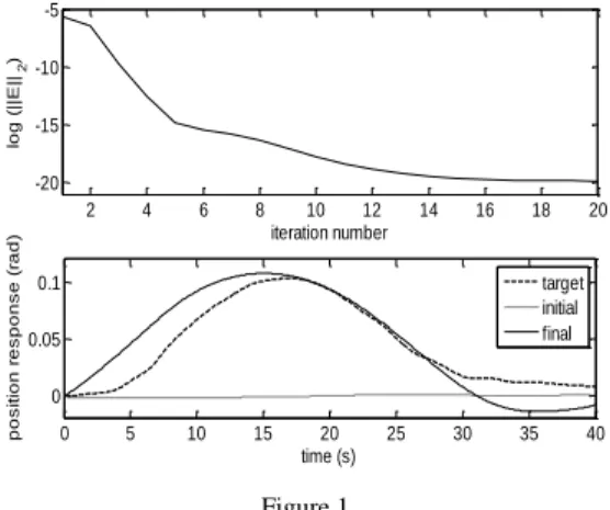
Q , where I is the general notation for th order identity matrix. The evolutions of the training error throughout the iterations and of the simulated trajectory before and after training are shown in Figure 1.
0 5 10 15 20 25 30 35 40 0
0.05 0.1
time (s)
position response (rad)
2 4 6 8 10 12 14 16 18 20
-20 -15 -10 -5
iteration number log (||E||2)
target initial final
Figure 1
NN training error versus iteration number and controlled output response before and after training
Two simulated case studies are next considered. The first simulated case study deals with the unconstrained optimization, where only the reference input signal is tuned according using our approach in order to ensure the output tracking improvement. A BFGS update was used for the Hessian estimate and the step size was chosen constant equal to 0.12. The final parameter vector that describes the reference input is
. ] 97.86 342.52
465.59 307.69
101.35 15.66 0.88 0.04
22 [
T
θ (34)
Figure 2 gives the initial and final reference input after optimization and the o.f.
decrease over the iterations. Only the first five parameters of the parameter vector are changed significantly. The control signal and the final controlled output before and after the optimization are shown in Figure 3 and in Figure 4, respectively. The rise of the reference input on the first 15 s with respect to the initial value and the decrease of the final reference input after 20 s compared to the initial reference input have to be correlated with the output response. This indicates that the reference input is tuned such as to anticipate the low bandwidth of the CS. As an effect, the final controlled output is rising faster under the take-off manoeuvre, and also tracks the reference input more accurately for the landing manoeuvre.