Remote reference magnetotelluric processing algorithm based on magnetic field correlation

O R I G I N A L S T U D Y

Remote reference magnetotelluric processing algorithm based on magnetic field correlation

Zhang Gang^1•Tuo Xianguo^1,2,3•Wang Xuben^3• Gao Song^3•Li Huailiang^1•Yu Nian^4•Liu Yong^1• Shen Tong¹

Received: 25 December 2016 / Accepted: 11 July 2017 / Published online: 20 July 2017 ÓAkade´miai Kiado´ 2017

Abstract Valid interpretations require precise and accurate determination of magne- totelluric impedance. Although remote reference magnetotellurics has been extensively investigated, majority of these studies have focused on the non-correlation between noise and signal or between the noise in the base station and that in the reference station. Few works have explored the correlation between magnetic signals in the base station and in the reference station. This study analyzes the effects of remote reference magnetotellurics on the sounding curve under different noise intensities in the base station. Results showed that regular remote reference magnetotellurics induce a limited quality-improving effect on the sounding curve and fail to satisfy the further data processing requirements at a low signal- to-noise ratio (SNR), suggesting that regular remote reference magnetotelluric methods cannot obtain an accurate transfer function under a lowSNRfor a time series. Comparison of various magnetic field data revealed that a strong correlation exists among magnetic signals 60 km apart at the Longmenshan area. Thus, the remote reference magnetotelluric method based on the magnetic field correlation between the base and reference stations is proposed to screen the power spectrum and undo the noise. The effectiveness and cor- rectness of the proposed method are validated by the results of the theoretical and field data processing and of the intermediate data analysis, further proving that the remote reference magnetotelluric method based on magnetic field correlation is superior to the regular remote reference magnetotelluric method.

Keywords Remote reference magnetotelluricsMagnetic field correlationTransfer functionSounding curveSignal-to-noise ratio

& Zhang Gang

zg@swust.edu.cn

1 School of Environment and Resource, Southwest University of Science and Technology, Mianyang 621010, China

2 Sichuan University of Science and Engineering, Zigong 643000, China

3 Institute of Geophysics, Chengdu University of Technology, Chengdu 610059, China

4

https://doi.org/10.1007/s40328-017-0203-y

1 Introduction

Magnetotelluric (MT) sounding method is a prominent approach for analyzing the electrical structure of the crust and the upper mantle. With the constant development of industrial society, electromagnetic instruments are recording increasingly severe noises. Thus, obtaining an unbiased estimation of the MT impedance tensor has become a pressing issue. At present, signal processing methods, such as wavelet transform (Trad and Travassos2000; Garcia and Jones2008), Hilbert–Huang transform (Cai2013), empirical mode decomposition (Neukirch and Garcia 2014), and statistical parameters (e.g., spectral power densities, coherences, response function distributions and their errors; Weckmann et al.2005), have been applied to effectively improve the signal-to-noise ratio (SNR) of the raw data in a time series. In the frequency domain, the sounding curve is significantly improved by robust estimation and remote reference processing. Robust estimation reduces the influence of the electric field noise on the tensor impedance, and remote reference processing eliminates the non-correlated noises between the base and remote stations. Egbert and Booker (1986), Chave et al. (1987), Larsen (1989), Sutarno and Vozoff (1991), and Smirnov (2003) applied robust theory to estimate magnetotelluric impedance. In this approach, the impedance obtained by least squares method is considered the initial impedance. The calculated electric field signal is compared with the measured electric field signal to obtain the residuals. Different weighting factors are then adopted according to the different residuals to reduce the field interference on the impedance result. Consequently, a more reliable sounding curve is achieved.

Remote reference magnetotellurics effectively eliminates non-correlated noises (Gam- ble et al.1979; Clarke et al.1983; Chave and Thomson1989; Ritter et al.1998; Oettinger et al.2001; Shalivahan et al.2006; Mun˜oz and Ritter2013). Gamble et al. (1979) analyzed the errors associated with remote reference and found that variances decreased as the number of measurements contained in the average powers increased. Egbert (1997) developed a robust multivariate errors-in-variables estimator that can automatically esti- mate incoherent noise levels. Shalivahan and Bhattacharya (2002) examined how the reference channel distance influenced the results of remote reference processing and found that the quality of the curves between 30 and 0.00055 Hz can be improved only if the reference station is more than 215 km away from the base station. Kappler (2012) iden- tified the time series spikes on the basis of inter-station comparisons within each time series window and replaced flagged windows with wiener filtering coincident data.

Given a local magnetic field H¼ðHx HyÞ, an electric field E¼ðEx EyÞ, and a reference station R, whose possible combinations are R¼ðExr EyrÞ or R¼ðHxr HyrÞ, among whichExr andEyr are observational electric fields of the refer- ence station andHxrandHyrare observational magnetic fields of the reference station, and given that the reference station is irrelevant to the noise signal of the local station, the equation of the calculated tensor impedanceZ¼ Zxx Zxy

Zyx Zyy

can be expressed as

Z¼ RyH 1

RyE

ð1Þ

In the equation,y represents the complex conjugate transpose,RyH andRyE are the cross powers. The signals recorded by the instruments represent the summation of effective signals and noises: E¼Es þEn,H¼Hs þ Hn, and R¼Rs þ Rn. Among them, Es

andEndenote the effective signals and noises of the electric field, respectively;HsandHn

represent the effective signals and noises of the magnetic field, respectively; R is the component of electric field or magnetic field of the reference station; andRsandRnare the

effective signals and noises of the reference field, respectively. Thus, Eq. (1) is trans- formed into

Z ¼ RyH1

RyE

¼hðRsþRnÞyðHsþHnÞi1

RsþRn

ð ÞyðEsþEnÞ h i

¼ Ry

sHsþRy

sHnþRy

nHsþRy

nHn

¹ Ry

sEsþRy

sEnþRy

nEsþRy

nEn

ð2Þ

The base station is irrelevant to the noise of the reference station. Therefore, Ry

nHs¼Ry

sHn¼Ry

nEs¼Ry

sEn¼0.

Equation (2) changes to Z¼ Ry

sHsþRy

nHn

¹ Ry

sEsþRy

nEn

, and the MT response obtained by linear systems analysis isEs¼HsZs,En¼HnZn, whereZsis the real tensor impedance. Thus,

Z¼ Ry

sHsþRy

nHn

1

Ry

sHsZsþRy

nHnZn

ð3Þ

The noises of the base and reference stations originate from different sources. There- fore,½Ry

nHn ¼0, and Eq. (3) changes to Z¼ Ry

sHs

¹ Ry

sHsZs

¼ Ry

sHs

¹ Ry

sEs

¼Zs ð4Þ

Equation (4) shows that after reference processing, the obtained tensor impedance is equal to the real tensor impedance, proving that remote reference magnetotellurics can effectively eliminate uncorrelated noise.

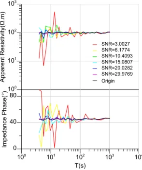
We simulate two 100 Ohm-m homogeneous half-space time series from the EMTF software package (Egbert1997). Noise with differentSNRsare added to theHychannel of the time series at the base station, and the remote reference processing results are shown in Fig.1.

Non-correlated noise is also added, as shown by the simulated results, and different processing effects are obtained under differentSNRs. Under a lowSNR(SNR=3.0027), the sounding curve is discontinuous in morphology. The sounding curve is improved as the SNRincreases. When the SNR reaches 29.9769, the sounding curves approach the origin curve, which does not contain noise.

The simulated results indicate that under a low SNR, regular remote reference pro- cessing cannot obtain an accurate transfer function, suggesting that regular remote refer- ence magnetotelluric methods cannot achieve an accurate transfer function under a low SNR for the time series. Thus, this paper proposes the use of magnetic field correlation between the base and reference stations to filter the data, suppress the noise, and improve the quality of magnetotelluric sounding curves.

2 Remote reference magnetotelluric processing method based on magnetic field correlation

2.1 Natural magnetic field correlation

Field data are acquired from the Xiaojin-Leshan survey line and from the China Geological

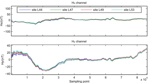
Figure3 depicts the time series of magnetic fields Hx andHy, and the four time syn- chronization sounding stations synchronously collect the electromagnetic field data by employing a GPS satellite. The starting and ending times are 0:00 GMT and 24:00 GMT, respectively. The sampling rate is 1 Hz, and the data collected in 1 day amounts to 86,400.

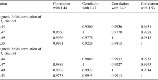
Figure3shows that in the four sounding stations, although the amplitudes of the magnetic fields fail to be consistent with one another, they maintain the same variation trend over time. The reason is that the field magnetic fluxgate is leveled manually, and the magne- tometer reacts sensitively to the changes in direction when magnetic data are received from HxandHy. To minimize the effects of human factors, such as the varying directions of the magnetic fluxgate, each channel data is subtracted from its mean value (DC component), and another time series indicating the change rule is obtained (Fig.4). The four curves hold the same shape and coincide with one another. The calculation result of the correlation of the magnetic fields in the four sounding stations (Table1) indicate that regardless of the magnetic field (Hx orHy), each magnetic field is highly correlated with the other three magnetic fields. This finding indicates the stability of the magnetic field and the homology of magnetic signals in this area even at the farthest distance of 60 km among the four sounding stations.

2.2 Algorithm

Formula (2) can be rewritten as follows:

Z¼RyH1

RyE

¼ Ry

sHsþRy

sHnþRy

nHsþRy

nHn

¹ Ry

sEsþRy

sEnþRy

nEsþRy

nEn

10⁰ 10¹ 10² 10³

Origin

10⁰ 10¹ 10² 10³ 10

0 Fig. 1 Hychannel is added with

differentSNRsnoises to obtain different sounding curves

Ry

nHn ¼Ry

sHn¼Ry

nHs¼0 is not completely true for areas with serious correlated interference for magnetic fields. In this situation, the tensor impedance calculated by Eq. (4) is a biased estimation. The relevant simulation results are illustrated by the sounding curve (SNR=3.0027) in Fig.1, which shows that the sounding curve is severely distorted.

Therefore, the magnetic field is evidently correlated in certain areas, as revealed by the analysis in Sect.2.1. The coherenceCohHibHir of the local magnetic fieldsHibandHircan be defined as follows:

CohHibHir¼X^N

k¼1

SHibHir

j j²_k SHibHibkSHirHirk

In the formula,iindicates the direction ofx andy,N is the sum of independent data segments, k is the sequence number of independent data segments, SHibHir is the cross- power spectrum of the base station magnetic fieldHiband the reference station magnetic fieldHir, andSHibHib is the auto-power spectrum of the base station magnetic fieldHib.

Chengdu

Guangyuan

Deyang Mianyang

Neijiang Suining

Leshan Meishan Ya an

Ziyang Maerkang

Kangding

Songpan

Xiaojing A ba

XS

Hf GLf

WL f

DSf SJSf

PGf BYf MW

f LRBf

ABf

LQSf L42 L44 L47 L49

L39 L36 L33

L29 L53

L67 L72 L81 L86 L89 L91

105˚

㠚䍑

MT station

>3>4 >5 >6

Hypocenter of Lushan Mw6 .6 earthquake Fault

Aftershock of Lushan City

0 3000 6000m

0 50 km100

Mw6.6 earthquake

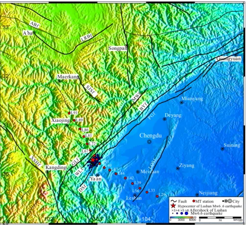
Fig. 2 Locations of the MT sounding stations. The faults taken from Deng et al. (2003), and reference 1:500,000 geological map database of the People’s Republic of China.LRBfLongriba fault,SJSfShuajinsi fault, MWf Maoxian-Wenxian fault, BYf Beichuan-Yinxiu fault; PGf Pengxian-Guanxian fault, LQSf Longquanshan fault,GLfGenda-Longdong fault,WLfWulong fault,DSfDachuan-Shuangshi fault

The specific process is described as follows:

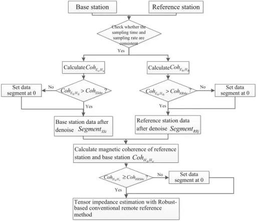
(1) Check and confirm the consistency of the sampling time and sampling rate of the data collection of the base and reference stations.

(2) Calculate the base station magnetic and electric coherence CohEsiHsj. If CohEsiHsjCohssthr (Cohssthr is the coherence threshold of the base station), keep and mark this data segment. Then, determine the data segmentSegmentSSiwhere the base station magnetic field is less interfered by noises.Coh_EsiHsj can be defined as follows:

2.95 3 3.05 3.1 3.15

x 10⁴

Hx/(nT)

Hx channel

site L44 site L47 site L49 site L53

1 2 3 4 5 6 7 8

x 10⁴

−150

−100

−50 0 50

Hy/(nT)

Sampling point Hy channel

Fig. 3 Time series of the magnetic fields in L44, L47, L49, and L53

0 50 100

Hx

site L53

1 2 3 5 6

x 10 0

20

Hy

Fig. 4 After deducted the direct current (DC) component, the time series comparison of the magnetic fields in L44, L47, L49, and L53

CohEsiHsj ¼X^N

k¼1

SEiHj

²_k S_EiEikS_HjHjk

In the formula,iandjindicate the directions ofxandy,Nis the sum of independent data segments,kis the sequence number of independent data segments,SEiHj is the cross-power spectrum ofEiandHj.

(3) Calculate the reference station magnetic and electric coherence CohERiHRj. If CohERiHRjCohRRthr (CohRRthr is the coherence threshold of the reference station), keep and mark the data segment. Then, obtain the data segmentSegmentRRjwhere the reference station magnetic field is less interfered by noises.

(4) Calculate the coherenceCohHibHirof the magnetic-field component inSegmentSSiand that in SegmentRRj. When CohHibHirCohHRSthr (CohHRSthr is the coherence threshold of the magnetic fields of the base and reference stations), proceed to step (6); otherwise, proceed to step (5).

(5) WhenCohH_ibH_ir\CohHRSthr, discard the data segment that is involved in the follow- up tensor estimation.

(6) Adopt the conventional robust estimation method for tensor impedance estimation.

Ideally,CohH_ibHir ¼1. In practical data processing, a lower interference of the magnetic field by noise corresponds to a higher coherenceCohH_ibH_ir. The data range ofCohH_ibH_ir is [0, 1]. The threshold ofCohHRSthrcan set range [0, 1], if the threshold ofCohHRSthris too small and the extreme valuesCohHRSthr¼0, the whole segments can meet the criteria and the algorithm become regular remote reference magnetotellurics, and if the threshold of CohHRSthr is too large and the extreme values CohHRSthr¼1, which results very small amount of segments to involved in the follow-up tensor estimation, obviously, bias esti- mation can obtained, so it is generally set toCohHRSthr¼0:8. WhenCohH_ibHir[CohHRSthr, it can be involved in the subsequent calculation; otherwise, the magnetic field receives unacceptable interference from the noises, and the data will be eliminated to reduce its influence on subsequent tensor estimations (Fig.5).

Table 1 Correlation of the Magnetic fields in L44, L47, L49, and L53

Station Correlation

with L44

Correlation with L47

Correlation with L49

Correlation with L53 Magnetic fields correlation of

Hxchannel

L44 1 0.9560 0.9936 0.9931

L47 0.9560 1 0.9778 0.9228

L49 0.9936 0.9778 1 0.9813

L53 0.9931 0.9228 0.9813 1

Magnetic fields correlation of Hychannel

L44 1 0.9889 0.9932 0.9758

L47 0.9889 1 0.9927 0.9943

L49 0.9932 0.9927 1 0.9914

L53 0.9758 0.9943 0.9914 1

3 Data experiments

3.1 Theoretical data experiment

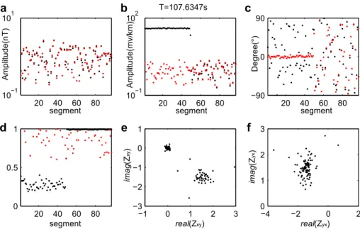
Figure6 provides the intermediate result data of the regular remote reference magne- totellurics. The theoretical data introduced in Sect.1is used in this experiment. The square wave noise is added to theHychannel at first half time series at the base station to illustrate the data processing in a period of 107.6347 s. The analyzed frequency band in the period of 107.6347 s ranges from 4 to 256 s, and the time window length at each segment is set to four times of the maximum period. Thus, each time series segment at the frequency band is 49256=1024 s. The overlapping ratio of each segment is set to 0.6. The black solid dot in Fig.6a, b represents the spectrums of theHxandHychannels at the base station. The red solid dot in Fig.6a, b represent the power spectrums of the Hx (Hx R) and Hy (Hy R) channels at the remote station. In Fig.6c, the black and red solid dots denote the polar- ization direction of the electric and magnetic fields, respectively. In Fig.6d, the black solid dot indicates the Hy correlation coefficient, and the red solid dot represents theHx cor- relation coefficient between the base and remote stations. Figure6e, f represent the scatter of the impedance tensor elementsZxyandZyx, and the horizontal and vertical axes at each scatter represent the real and image parts of each tensor, respectively.

Base station Reference station

Calculate

si sj

CohE H CalculateCohE H_{Ri Rj}

> ?

Si Sj E H CohSSthr

Coh CohE H_{Ri Rj}>CohRRthr?

Reference station data after denoise Base station data after

denoise

Tensor impedance estimation with Robust- based conventional remote reference method

Check whether the sampling time and sampling rate are

consistent Yes

Yes

Set data segment at 0 No

Set data segment at 0 Set data

segment at 0

Yes Yes

No No

SegmentSSi SegmentRRj

Calculate magnetic coherence of reference station and base station

ib ir ?

H H CohHRSthr

Coh ≥

ib ir

CohH H

Fig. 5 Flow chart of remote reference magnetotelluric data processing based on magnetic coherence

In the standard time series without any noise, theHx,Hx R(Fig.6a), andHy R(Fig.6b, red dot) channels have small power spectrum values. However, in theHy (Fig.6b, black dot) channel with noise interference, the first half of the power spectrum is strongly interfered, and its amplitude is at least two to three orders of magnitude larger than the regular amplitude. The magnetic field polarization direction (Fig.6c red dot) also shows that the first half displays great consistency, which is inconsistent with the unordered law of natural magnetotelluric signal polarization direction (Weckmann et al. 2005). The magnetic fields from the base stations to the reference stations maintain a low correlation within 0.2–0.4 in the first half (Fig.6d, black dot), but they encounter interference in the latter half with a high correlation of nearly 1. The impedance tensorZxypresents multiple dispersed values with two aggregations: one is near (0, 0) and the other is near (1.5,-1.5).

Thus, the sounding curve deviates from the true value and yields a breakdown point at a period of 107.6347 s (Fig.8a,xydirection of the sounding curve). However, given that no noise is added to theHx channel, the scatter of the impedanceZyxis only one aggregation (Fig.6f). Consequently, smooth curves are obtained at the period (Fig.8a,yxdirection of the sounding curve).

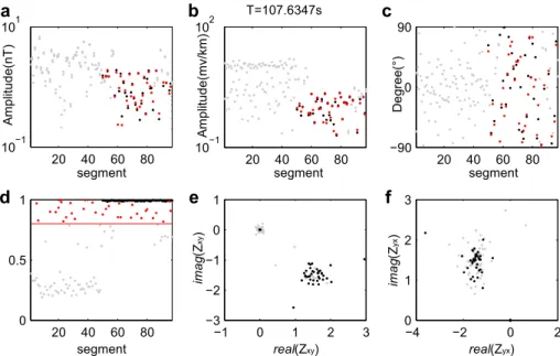
As shown in Fig.4and Table1, a magnetic field is correlated with another in a certain range. Therefore, the correlation between the magnetic fields in the base and reference stations can be used to detect the noise level of the magnetic field. A higher correlation indicates less interference of the magnetic field, whereas a lower correlation indicates a higher interference of the magnetic field. Furthermore, the data with a low correlation can be removed to mitigate the impact on future calculations of tensor impedance and con- sequently improve the quality of the sounding curve. Figure7shows the intermediate data

20 60

10 10¹

20 60

10 10²

20 60

0

20 60

0 1

0 1 2 3

0 1

0 2

0 1 2 3

real(Zxy real(Zyx

imag(Zxy imag(Zyx

a b c

d e f

Fig. 6 Intermediate data with regular remote reference magnetotelluric method (T=107.6347 s).aBlack dotspectra ofHxchannel at base station (Hx),red dotspectra ofHxchannel at remote station (Hx R);b black dotspectra ofHychannel at base station (Hy),red dotspectra ofHychannel at remote station (Hy R);c black dot electric field polarization direction,red dotmagnetic field polarization direction;dblack dot correlation coefficient betweenHyandHy R,red dotcorrelation coefficient betweenHxandHx R;escatter of impedance tensor elementZxy;fscatter of impedance tensor elementZyx. (Color figure online)

in the period of 107.6347 s by using the correlation between the magnetic fields in the base and reference stations. As shown in Fig.6e, the interference of the square wave noise causes the magnetic fields from the base and reference stations to maintain a low corre- lation (from 0.2 to 0.4) in the first half of the data segment. The correlation approaches to 1 in the latter half. The threshold value is set to 0.8 (Fig.7d; the data is removed if the correlation coefficient is below 0.8; the gray dot represents the removal of data) to remove the first half of the data segment interfered by the noise. Figure7a, b show the electric and magnetic field spectra after the data removal (the gray dot represents the removed data).

After the noise data is removed, the polarization direction scatter shows disorder in the entire period; this behavior is consistent with the characteristic of natural magnetotelluric data (Weckmann et al. 2005). The scatter of Zxy shows it retains only one aggregation, causing the sounding curves to become smoother (Fig.8b) than that obtained by regular remote reference methods (Fig.8a).

3.2 Field data experiment

The measured data is used as the time series data of the sounding station L44 in Sect.2.1.

The Lemi-417 instrument is utilized with a sampling rate of 1 Hz (fs=1 Hz), and the time series obtains 1,209,600 samples after 14 days of data collection. Five components of observation data, namely,Ex,Ey,Hx,Hy, andHz, are obtained. The reference station L39 collects the time series of the electromagnetic field at the same time with its base station by GPS synchronization, and its sampling rate is set as the same with that of L44.

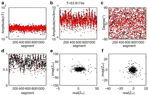
Figure9shows the intermediate results of the conventional remote reference magne- totelluric processing at 53.8174 s. The overlap rate of each time window is set to 0.33. The power spectrum of the base station Hx and the reference station Hx R (Fig.9a) and the

20 60

10 10¹

20 60

10 10²

20 60

0

20 60

0 1

0 1 2 3

0 1

0 2

0 1 2 3

real(Zxy real(Zyx

imag(Zxy imag(Zyx

a b c

d e f

Fig. 7 Intermediate data with remote reference magnetotelluric processing algorithm based on magnetic field correlation (T=107.6347 s). Thegray dotrepresents the rejection of the noise data with magnetic field correlation; the other legend labels are consistent with those in Fig.6

power spectrum of the base stationHy and the reference stationHy R (Fig.9b) are cal- culated. The fluctuation and shape of the power spectrum of the base and reference stations are consistent, whereas the power spectrum of some frequencies differ. Although the polarization direction of the electromagnetic field (Fig.9c) is messy and consistent with the characteristic of natural magnetotelluric data, the contamination of the segment cannot be assessed. The calculation results of the magnetic coherence between the base and reference stations (Fig.9d) show that the magnetic coherence at some data segments is below 0.3, indicating that the magnetic field in these data segments are interfered by noise.

Under this condition, the elements of tensor impedanceZxy andZyxare scattered (Fig.9e, f).

According to the correlation principle between the tracks of the base and reference stations, the threshold is set to 0.8, and the data segment below the threshold is detected (gray dots in Fig.10d), indicating that the data segment receives an unacceptable noise interference. The magnetic coherence detects the data segment (gray dots in Fig.10c) where the polarization direction of the electric and magnetic fields cannot be detected. The power spectrum of this data segment is eliminated and ignored in subsequent tensor impedance calculations (gray dots in Fig.10a, b). The scatter diagram of the elements of tensor impedanceZxyandZyxshows that the previous scattered data interfered by noises are eliminated (gray dots in Fig.9e, f), and the remaining data are concentrated (black dots in Fig.9e, f). The clustered data guarantees that reliable sounding curves can be acquired.

10⁰ 10¹ 10² 10³

10 ρ_xy

ρ_yx

10¹ 10² 10³ 0

φxy

φyx

10^-1 10⁰ 10¹ 10² 10³

10¹ 10² 10³ 0

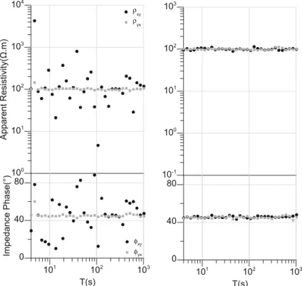
Fig. 8 Comparison between the regular remote reference method and the remote reference method based on magnetic field correlation under the interference of square wave.Left columnregular remote reference method result,right columnremote reference method based on magnetic field correlation result

200 600 1000 10

10⁰

200 600 1000 10

10

200 600 1000 0

200 600 1000 0

1

0 50

0 0 50 100

0 20

0 20

real(Z^xy real(Z^yx

imag(Zxy imag(Zyx

a b c

d e f

Fig. 9 Intermediate data of L44 station with regular remote reference magnetotelluric method (T=53.8174 s). The legend labels are consistent with those in Fig.6

200 600 1000 10

10⁰

200 600 1000 10

10

200 600 1000 0

200 600 1000 0

1

0 0 50

0 0 50 100

0 20

0 20

real(Zxy real(Zyx

imag(Zxy imag(Zyx

a b c

d e f

Fig. 10 Intermediate data of L44 station with remote reference magnetotelluric processing algorithm based on magnetic field correlation (T=53.8174 s). Thegray dotrepresents the rejection of the noise data with magnetic field correlation; the other legend labels are consistent with those in Fig.6

2SpectrascreeningresultofL44soundingstationwithremotereferencemagnetotelluricsmethodbasedonmagneticcoherence Frequency band(T/s)Segment amountSegmentremove amountProportionofremove segmentVarianceofZxy beforefilterVarianceofZxy afterfilterVarianceofZyx beforefilterVarianceofZyx afterfilter 1744–25611758060.68598.75953.63373.86522.0607 634732–5125872100.35786.00095.30192.94731.8406 269564–1024293810.27653.96143.85201.76551.6622 0779128–40967380.10960.88220.87320.63820.5031 .1559512–81923640.11110.66890.67730.25970.1706 .31171024–16,3841820.11111.00720.96430.50300.1654

The entire period of the frequency band is 4–16,384 s. To increase the superposition times of the sub-spectra and thus achieve accurate estimation, six sub-frequency bands, namely, 4–256, 128–512, 256–1024, 512–4096, 1024–8192, and 4096–16,384 s, are divided. After the power spectrum is computed for each subband, data screening is con- ducted based on the established rules. The specific screening results are shown in Table2.

As shown, the highest proportion of eliminated data segments in the high-frequency part is up to 0.6859, whereas most of the data segments in low-frequency part are preserved. In the last two subbands, the proportion of eliminated data segments is only 0.1111. This result indicates that the magnetic field in this test station is more severely interfered at the high-frequency part than that at the low-frequency part. Remote reference magnetotelluric processing based on magnetic coherence is adopted to summarize the variance before and after data screening. Before screening, the variances of Zxy and Zyx in the high-frequency part are 8.7595 and 3.8652, which are reduced to 3.6337 and 2.0607 after screening. The tensor impedance variances in the other subbands are also decreased (Table2).

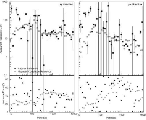
Figure11 shows the comparison of processing results obtained by the conventional remote reference method and the remote reference method based on magnetic coherence at the L44 station. The black solid dot represents the conventional remote reference pro- cessing, and the gray dot line denotes the remote reference processing based on the magnetic coherence. The sounding curve of the conventional remote reference processing is messy and cannot be used for subsequent inversion. After remote reference processing based on magnetic coherence is performed, the sounding curve becomes more continuous in morphology.

1 10 100 1000

10 100 1000 10000

0 20 60

10 100 1000 10000

Aapparent Resistivity(

yx direction xy direction

Fig. 11 Comparison of processing results obtained by different methods at L44 station

4 Conclusions

This paper explains the principle of conventional remote reference magnetotelluric methods by analyzing the simulation data. The effects of conventional remote reference magnetotellurics on the sounding curve are simulated under different noise intensities.

According to the coherence calculation of the magnetic field in the Longmenshan area, the magnetic fields between two stations that are 60 km apart have good correlation. Thus, a remote reference magnetotelluric method based on magnetic coherence is proposed for processing magnetotelluric data. The following conclusions are drawn:

1. Conventional remote reference magnetotellurics can improve the quality of sounding curves. Under a lowSNR(SNR=3.0027 dB), the noise covers the useful signals, and the influence of remote reference magnetotellurics on the sounding curve is limited.

Thus, it cannot meet the demand of follow-up data processing. Under a high SNR (SNR=29.9769 dB), remote reference magnetotellurics can restore the true apparent resistivity;

2. At a distance of 60 km in the Longmenshan area, the magnetic field is stable in a certain range, and a high coherence is exhibited by the magnetic field data collected at different stations. Therefore, the magnetic coherence at the base and reference stations is adopted to determine the degree of interference and eliminate the electromagnetic spectrum of the data segment severely interfered by noise (the coherence threshold in this study is set to 0.8). Consequently, this data segment is rejected from the tensor impedance calculation, thereby enhancing the quality of the sounding curve.

3. The remote reference calculation method based on magnetic coherence requires that the magnetic field noise at the reference and base stations is uncorrelated. Therefore, when setting the stations, the reference station should be placed far away enough from the base station to prevent them from being interfered by homologous noise.

Acknowledgements This study was supported by the China Postdoctoral Science Foundation (Grant 2017M610611), Natural Science Funds of Southwest University of Science and Technology (Grant 15zx7135), the National High Technology Research and Development Program of China (Grant 2014AA06A612), Chinese National Natural Science Foundation (Grant 41504061). We also thank editor Dr. Endre Turai and two anonymous reviewers for their detailed comments that helped us improve the quality of the manuscript.

References

Cai JH (2013) Magnetotelluric response function estimation based on Hilbert–Huang transform. Pure Appl Geophys 170(11):1899–1911

Chave AD, Thomson DJ (1989) Some comments on magnetotelluric response function estimation. J Geo- phys Res 94(B10):14215–14225

Chave AD, Thomson DJ, Ander ME (1987) On the robust estimation of power spectra, coherences, and transfer functions. J Geophys Res Solid Earth 92(B1):633–648

Clarke J, Gamble TD, Goubau WM et al (1983) Remote-reference magnetotellurics: equipment and pro- cedures. Geophys Prospect 31(1):149–170

Deng Q, Zhang P, Ran Y, Yang X, Min W, Chu Q (2003) Basic characteristics of active tectonics of China.

Sci China (Ser D Earth Sci) 46:356–372

Egbert GD (1997) Robust multiple-station magnetotelluric data processing. Geophys J Int 130(2):475–496 Egbert GD, Booker JR (1986) Robust estimation of geomagnetic transfer functions. Geophys J R Astron Soc

87(1):173–194

Gamble TD, Goubau WM, Clarke J (1979) Magnetotellurics with a remote reference. Geophysics 44(1):53–68

Garcia X, Jones AG (2008) Robust processing of magnetotelluric data in the AMT dead band using the continuous wavelet transform. Geophysics 73(6):F223

Kappler KN (2012) A data variance technique for automated despiking of magnetotelluric data with a remote reference. Geophys Prospect 60(1):179–191

Larsen JC (1989) Transfer functions: smooth robust estimates by least-squares and remote reference methods. Geophys J Int 99(3):645–663

Mun˜oz G, Ritter O (2013) Pseudo-remote reference processing of magnetotelluric data: a fast and efficient data acquisition scheme for local arrays. Geophys Prospect 61:300–316

Neukirch M, Garcia X (2014) Nonstationary magnetotelluric data processing with instantaneous parameter.

J Geophys Res Solid Earth 119:1634–1654

Oettinger G, Haak V, Larsen JC (2001) Noise reduction in magnetotelluric time-series with a new signal–

noise separation method and its application to a field experiment in the Saxonian Granulite Massif.

Geophys J Int 146(3):659–669

Ritter O, Junge A, Dawes G (1998) New equipment and processing for magnetotelluric remote reference observations. Geophys J Int 132(3):535–548

Shalivahan, Bhattacharya BB (2002) How remote can the far remote reference site for magnetotelluric measurements be? J Geophys Res Atmos 107(B6):1

Shalivahan, Sinharay RK, Bhattacharya BB (2006) Remote reference magnetotelluric impedance estimation of wideband data using hybrid algorithm. J Geophys Res Solid Earth 111(B11):B11103

Smirnov MY (2003) Magnetotelluric data processing with a robust statistical procedure having a high breakdown point. Geophys J Int 152(1):1–7

Sutarno D, Vozoff K (1991) Phase-smoothed robust M-estimation of magnetotelluric impedance functions.

Geophysics 56(12):1999–2007

Trad DO, Travassos JM (2000) Wavelet filtering of magnetotelluric data. Geophysics 65(2):482 Weckmann U, Magunia A, Ritter O (2005) Effective noise separation for magnetotelluric single site data

processing using a frequency domain selection scheme. Geophys J Int 161(3):635–652