Is gold a safe haven? The international evidence revisited
LEVENT BULUT
1pand ISLAM RIZVANOGHLU
21Department of Economics and Finance, Harley Langdale, Jr. College of Business Administration, Valdosta State University, GA 31698, USA
2Department of Economics, University of Houston, TX, USA
Received: October 18, 2018 • Revised manuscript received: April 23, 2019 • Accepted: May 30, 2019
© 2020 Akademiai Kiado, Budapest
ABSTRACT
The literature has not settled down on safe haven property of gold in the emerging and developing countries. Therefore, we revisit the international evidence on hedging and safe haven role of gold for 34 emerging and developing countries with a span of daily data covering January 2000–November 2018. We employ the GARCH-copula approach to estimate the lower-tail extreme dependencies of the joint dis- tribution of gold and equity returns. We also introduce a new definition for the strong safe haven property of an asset. Our findings indicate that while gold serves as a hedging instrument for all countries in our sample, we got evidence of weak safe haven property for gold, for domestic investors, only in 20 countries, and a strong safe haven asset (SHA) only in 9 countries.
KEYWORDS
gold, emerging markets, copula, tail dependence, safe haven
JEL CLASSIFICATION INDICES C58, F30, G10, G15
1. INTRODUCTION
In recent years, the world economy experienced the worst global financial and economic turmoil since the Great Depression. Given the fact that the economies and markets are more integrated
pCorresponding author. E-mail: lbulut@valdosta.edu
than ever, and we have look-alike countries whose currencies and financial markets are moving together, there is an increasing demand amongst investors to seek for a safe haven asset (SHA) at the episodes of economic and financial calamities. The severity of the 2007 financial crisis and the threat of future unpredictable recessions provide a strong motivation for an investigation of a SHA.1
A SHA is defined as an investment instrument that shows zero or negative correlation with other assets in the periods of severe market turmoil. This way, investors that hold a true SHA in their portfolios will shield themselves from extreme losses. To capture this we need to analyze the co-movement between that instrument and other assets in the portfolio at extreme market falls. One motivation for the investors to seek SHA is to minimize risk exposure by having more good quality assets during severe market downturns, which is also known as the flight-to-quality phenomenon. Another motivation is to have greater liquidity during extreme market falls by having more true SHA, also known as the flight-to-liquidity phenomenon.
Additionally, we might have some institutional demand for gold by central banks or the government sector during turbulent times for purposes of strengthening current account sus- tainability, reducing the risk of sudden capital reversals, and increasing central banks’ “war- chest”. Especially for the emerging and developing countries, gold is seen as the ultimate asset to hold at times of high uncertainty. Therefore, central banks increase their reserves with gold to protect their countries from possible currency orfinancial crises. Given the stylized fact that gold and US dollar are negatively correlated, gold holdings also provide diversification for central banks that hold US dollars as reserves.2All these factors, in the case of gold, contribute to the hike in the gold price during market turmoil. In that regard, the relationship between gold and the stock market has historically been an intriguing one; a number of publications have been put forth as researchers attempt to delineate the role gold play as a SHA against different currencies and stock market indices.3From many aspects, gold can be considered as a natural candidate for SHA. In both advanced and emerging nations, whenever there is afinancial distress, we observe a spontaneous attack in the market to buy gold by both retail and professional investors. Also, increasing integration offinancial markets leads to synchronization of stock markets across the globe. As a result, at the times of market turmoil, it is not uncommon to see co-movements of different asset classes in the same direction. Since predictability and stability become crucial for investors at severe market downturns, gold’s safe-haven asset qualities shine as a universal safe- haven for preserving wealth.
There is almost a consensus that gold is a true SHA for the advanced economies’ stock markets. Baur – Lucey (2010) and Baur – McDermott (2010) found that, except for Australia, Canada, and Japan, this is true for the major European stock markets and the US.
Ciner et al. (2013), Reboredo (2013), Flavin et al. (2014), Beckman et al. (2015), Bredin et al.
1The unfolding COVID-19 crisis is the most recent example (Editor’s note).
2After thefinancial crises in 2008, the developed countries lowered their gold holdings while central banks of the emerging and developing countries did the opposite. One explanation would be that, due to the easy monetary policies of the advanced nations, the massive influx of money into the emerging and developing countries might have worried the recipient governments about a sudden reversal in their currencies.
3Baur–Lucey (2010), Ciner et al. (2013), Hood and Malik (2013) and Aboura et al. (2016)looked at the US markets.
Baur–Lucey (2010) and Baur–McDermott (2010)looked at the European markets.
(2015), and Liu (2019)confirmed the safe-haven feature of gold for the advanced economies.
However, when it comes to equity markets in the emerging and developing countries, there are mixed results. WhileBaur–McDermott (2010) and Bekiros et al. (2017)found that gold is not a SHA for the large emerging markets such as the BRICS countries,4Chkili (2016), on the other hand, using an asymmetric dynamic conditional correlation approach, reached an opposite conclusion. In a very recent article,Wen–Cheng (2018)found evidence in favor of safe haven role of gold against a small set of emerging nation stock market indices. On the other hand, by extending the analysis of Baur – McDermott (2010) to a sample of 28 emerging and developing countries, Gurgun – Unalmis (2014) reached an opposite conclusion when more data points are utilized. There are also some recent papers that found mixed evidence for the sample of the emerging and developing countries (Ahmed – Vveinhardt 2018).Beckmann et al. (2015)adopted a smooth-transition regression andfind an evidence of safe haven role for gold against stock indices but their results are country- specific. In the light of the previousfindings, we revisit the international evidence on safe haven role of gold. Our contribution to the literature is two-fold. First, we tested safe haven property for a broader sample of 34 emerging and developing countries with daily data spans from January of 2000 till November of 2018. Second, we utilize copulas which allow measuring the degree of association at a different part of the distribution so that we can focus only on the degree of association at extreme market conditions, not from central observations. Thecopula approach has the limitation that it can only be used to test weak safe haven property as it provides a non-zero probability of extreme price movements to test for non-correlated series. We propose applying Monte Carlo simulations on the best-fitting copula to properly test the degree of association for testing the strong safe-haven feature of gold.
The previous studies mostly use either linear threshold regression (Baur –McDermott 2010) or copula-based joint tail modeling (Reboredo 2013) techniques. The former relies on the average measure of dependencies at specific lower quantile levels, generally in between 5 and 1% lower quantile levels. However, as put forward byReboredo (2013), if there is any tail dependency between gold and stock returns, linear threshold regression approach will not be able to capture it properly, since extreme failures of the market don’t happen 5% of the time, 1% of the time, or even 0.001% of the time. We, therefore, model joint extreme movements of gold and equity returns with the use of copula and test the safe-haven feature of gold in 34 developing and emerging economies.5 Ourfindings indicate that while gold serves as a hedge instrument for all countries in our sample, we got evidence of weak safe haven property for gold only for 20 out of 34 countries and a strong safe haven only for 9 countries.
We organize the remaining parts as follows: In Section 2, we talk about our empirical methodology. Then in Section 3, we summarize data and provide descriptive statistics. We present ourfindings in Section 4 and conclude in Section 5.
4Brazil, Russia, India, China.
5We followReboredo (2013), Yang–Hamori (2014) and Reboredo–Ugolini (2015)in our approach. These papers examined the role of gold as a SHA against the developed economies stock market returns and currencies, however, we focus on the emerging market and developing economies.
2. METHODOLOGY
2.1. Modeling tail dependence
Earlier studies that use threshold regression models generally look at the correlation of investment instrument with a candidate of SHA at specific lower quantile levels, generally in between 5 and 1% lower quantile levels. The problem with this approach is the arbitrary nature of these per- centages. Extreme failures of the market don’t happen 5% of the time, 1% of the time, or even 0.001% of the time. Such catastrophes are almost impossible to predict in a systematic way and trying to capture this rare event with a linear regression model leave the researchers with too few data point to reach a meaningful conclusion. The copula-based approach, on the other hand, helps us to look at the dependence structure of two variables at the extreme cases, independent from how the marginal distributions are modeled. Even in the hypothetical scenario that both gold and stock returns have the same univariate distribution function, one cannot look at the corresponding tail dependency for the corresponding bivariate distribution function unless both series have the same tail heaviness in their marginal distributions. Copulas help us to avoid this problem by allowing different characteristics for marginal distributions. One can independently model the margins and the dependence structure and define the conditional distribution with the copula.
According to the Sklar’s theorem (Sklar 1959), any multivariate distribution can be rep- resented through its marginal distributions and a copula function. Given thatF1(x)5P[X≤x]
andF2(y)5P[Y≤y] are the cumulative distribution functions forXandYrespectively and F(x,y)5P[X≤x,Y≤y] being the joint distribution function of these two random variables, then a copula functionCis defined such thatF(x,y)5C(F1(x),F2(y)). In other words, copula functionCmaps marginal distributions to the multivariate distribution function. Denoting the probabilities u 5 F1(x) and v 5 F2(y), the Sklar’s theorem proposes that the copula of the joint distribution function for X and Y can be extracted as follows:
Fðx;yÞ ¼FðF1−1ðuÞ;F2−1ðvÞÞ ¼Cðu;vÞ, whereF1−1ðuÞandF2−1ðvÞare the quantile functions of the marginals for X andY.6 Accordingly, if we know C, then we can derive the joint distri- bution function,F(x,y), from the marginal distributions,F1(x) andF2(y).
Since we are interested in how the return series for gold and equities are correlated in times of stress, we need to measure the amount of dependence in the lower quadrant tail of the joint distri- bution of gold and equity returns. Hence, we use copulas to measure the bivariate tail dependence.
More specifically, we use the coefficient of lower tail dependence to measure the probability of observing small values ofYwhenXtakes a small value and we define lower-tail dependence as follows:
λL¼lim
a→0P Y≤F2−1ðaÞjX≤F−11 ðaÞ
(1) Likewise, the upper tail dependence coefficient measures the probability of observing a largeY given that Xtakes a large value and it is defined as follows:
λU ¼lim
a→1P Y≥F−21ðaÞjX≥F1−1ðaÞ
(2)
6The conditional distribution of Y given X variate takes the value of x can be written as follows:Fy|x(y)5C1(Fx(x),Fy(y)) where theC1is thefirst partial derivative of the copula.
2.2. Weak and strong safe-haven property
By definition, if two assets exhibit negative or zero correlation on average, they are considered to be appropriate hedge instruments for each other. For safe haven property, we need to know whether these two assets are negatively (or un-)correlated during the extreme market con- ditions. In our specific case, we want to find out if a domestic investor in our sample countries can retain the value of their gold holdings during a stock market crash. However, standard correlation coefficients are only the average measures. Alternatively, one can set an exogenous threshold for the lower tail and calculate the correlation for that part of the data only. This approach is technically the intuition behind the threshold regression method used byBaur –McDermott (2010)and others. Since we have a very limited number of observa- tions to analyze market behavior at extreme market conditions, the threshold regression approach may fail to correctly measure dependencies at extremely rare events. So, we look at the possibility of simultaneous extremes by looking at the tail of the distribution of losses by the copula-based approach. However, by using this method, we can only calculate the con- ditional probability of losses, rather than the correlation, inY(gold in our case), given thatX (equities in our case) is also experiencing a big downturn. We follow the literature and define a weak SHA as an investment instrument that shows zero lower tail dependence with another asset (whenλL50). In other words, if gold is a weak safe haven instrument, an investor will experience no loss in his/her gold holdings during the stock market crashes. On the other hand, a positive lower-tail distribution (λL> 0) implies that there is a positive probability of concurrent losses in gold and equities at market turmoils. Since λL is only a conditional probability measure, rather than a tail correlation, havingλL> 0 does not necessarily imply zero probability of positive gold returns in the event of big losses in equities. More specif- ically, regardless of the value ofλL, it is still possible for gold to offer positive returns when equities are at an extreme loss. We define this situation with a negative correlation between stock market (X) and gold (Y) returns at the lower tail of stock returns distribution,r(X,Y|X
<Xq) < 0, where Xq denotesqth percentile ofX.
Intuitively, even though havingr(X,Y|X<Xq) < 0 is much desired feature on a SHA, it is still risky to hold two assets withr(X,Y|X<Xq) < 0 if theirλLis also positive. Given this rationale, we propose the following conditions for strong safe-haven property: an asset is said to have a strong safe haven property only ifλL50 andr(X,Y|X<Xq) < 0 hold at the same time. Having r(X,Y|X <Xq) < 0 is necessary, but definitely not a sufficient condition for strong safe haven property.
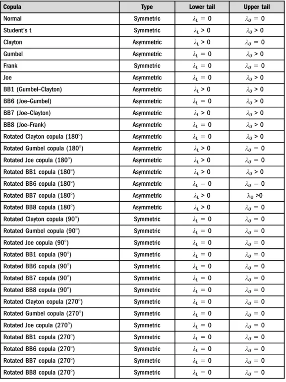
We fit 39 different types of copula functions7to find the best one for the tail dependence between the stock market and gold returns. Each copula function has a different structure of low and high tail dependencies. For example, as shown inTable 1, Normal, Gaussian, Plackett and Frankel copulas have no tail dependency (λL5 λU5 0) which can give us information about being a weak SHA. Clayton copula has only lower tail dependence and zero dependence on the upper tail (λL> 0,λU 50). Gumbel copula has only upper tail dependence (λL50, λU> 0).
Student’s t copulas, derived from the multivariate t-distribution, have symmetric and positive tail dependence (λL> 0,λU> 0). As shown inTable 2, stock and gold returns exhibit a negative
7SeeBrechmann–Schepsmeier (2013)for more details.
Table 1. Copula functions and their implied tail dependence parameters
Copula Type Lower tail Upper tail
Normal Symmetric λL50 λU50
Student’s t Symmetric λL> 0 λU> 0
Clayton Asymmetric λL> 0 λU50
Gumbel Asymmetric λL50 λU> 0
Frank Symmetric λL50 λU50
Joe Asymmetric λL50 λU> 0
BB1 (Gumbel–Clayton) Asymmetric λL> 0 λU> 0
BB6 (Joe–Gumbel) Asymmetric λL50 λU> 0
BB7 (Joe–Clayton) Asymmetric λL> 0 λU> 0
BB8 (Joe–Frank) Asymmetric λL50 λU> 0
Rotated Clayton copula (1808) Asymmetric λL50 λU> 0
Rotated Gumbel copula (1808) Asymmetric λL> 0 λU50
Rotated Joe copula (1808) Asymmetric λL> 0 λU50
Rotated BB1 copula (1808) Asymmetric λL> 0 λU> 0
Rotated BB6 copula (1808) Asymmetric λL50 λU50
Rotated BB7 copula (1808) Asymmetric λL> 0 λU>0
Rotated BB8 copula (1808) Asymmetric λL> 0 λU50
Rotated Clayton copula (908) Symmetric λL50 λU50
Rotated Gumbel copula (908) Symmetric λL50 λU50
Rotated Joe copula (908) Symmetric λL50 λU50
Rotated BB1 copula (908) Symmetric λL50 λU50
Rotated BB6 copula (908) Symmetric λL50 λU50
Rotated BB7 copula (908) Symmetric λL50 λU50
Rotated BB8 copula (908) Symmetric λL50 λU50
Rotated Clayton copula (2708) Symmetric λL50 λU50
Rotated Gumbel copula (2708) Symmetric λL50 λU50
Rotated Joe copula (2708) Symmetric λL50 λU50
Rotated BB1 copula (2708) Symmetric λL50 λU50
Rotated BB6 copula (2708) Symmetric λL50 λU50
Rotated BB7 copula (2708) Symmetric λL50 λU50
Rotated BB8 copula (2708) Symmetric λL50 λU50
(continued)
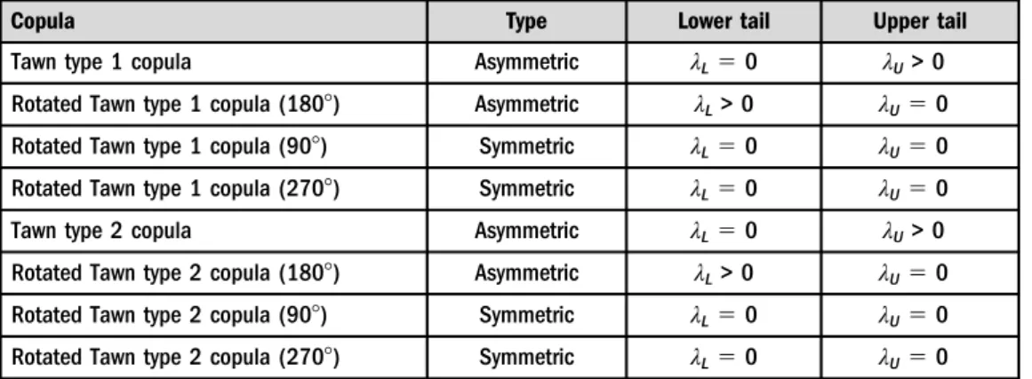
correlation in 21 countries in our sample. Where there is an empirical negative correlation in the data, copulas such as Clayton’s copula, Gumbel’s copula and Frank’s copula would not be able to capture the negative dependency. Therefore, these copulas needed to be rotated to avoid forcing empirical results to Student’s t copula. Hence, we employ 39 different types of copulas in our study to be able to yield any kind of dependence structure in the data. We only focus on static copulas as time-varying copulas do not always provide a betterfit than static copulas.8
3. DATA, COUNTRY COVERAGE, AND DESCRIPTIVE STATISTICS
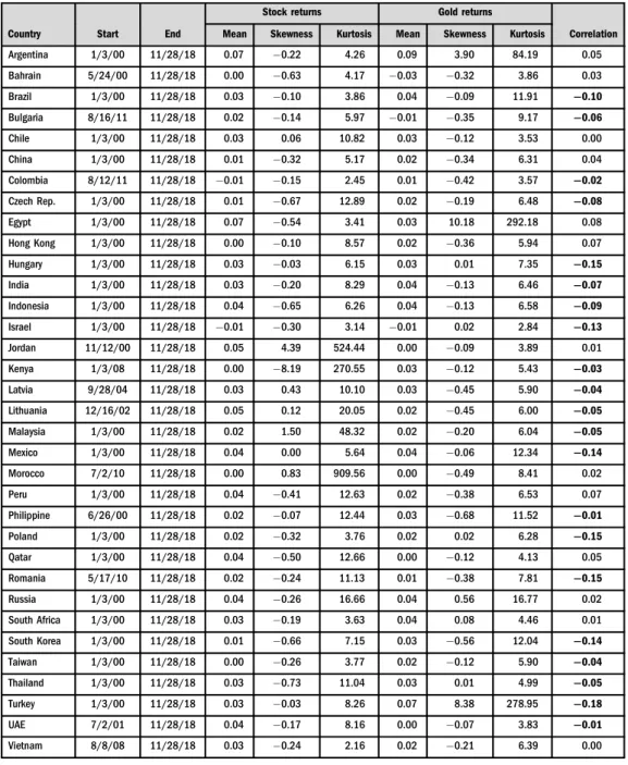
We have 34 emerging market economies in our sample and our daily data cover the period from January 4, 2000 till November 28, 2018.Table 2 reports the summary statistics of the daily logarithmic returns on domestic stock indices and gold9in domestic currency. Equity markets on average have 2.6% annualized daily return, while gold offers a higher annualized daily return at 2.9%. Majority of the countries in our sample have negative skewness in their distribution of stock return series which indicates that there is a likelihood of extreme loss occurrences in these countries. Besides, for all countries in the sample, high kurtosis numbers point to the existence of extreme stock market returns observed at relatively high frequencies. As for the gold return in domestic currency, we see that majority of the countries have left-skewed distribution for gold returns, except for Argentina, Egypt, Israel, Poland, Russia, South Africa, Thailand and Turkey.
Hence, we can infer that in the sample, we have high probabilities of extreme loss or gain occurrences for gold return.
Table 1.Continued
Copula Type Lower tail Upper tail
Tawn type 1 copula Asymmetric λL50 λU> 0
Rotated Tawn type 1 copula (1808) Asymmetric λL> 0 λU50
Rotated Tawn type 1 copula (908) Symmetric λL50 λU50
Rotated Tawn type 1 copula (2708) Symmetric λL50 λU50
Tawn type 2 copula Asymmetric λL50 λU> 0
Rotated Tawn type 2 copula (1808) Asymmetric λL> 0 λU50
Rotated Tawn type 2 copula (908) Symmetric λL50 λU50
Rotated Tawn type 2 copula (2708) Symmetric λL50 λU50
Notes:The table shows the behavior of 39 selected copulas in the right and left tails.λLandλUrefer to lower tail and upper tail dependence, respectively.
8SeeBekiros et al. (2017)for detail.
9We use gold price in each country to calculate the return on gold.
Table 2. Summary statistics of stock and gold returns
Stock returns Gold returns
Country Start End Mean Skewness Kurtosis Mean Skewness Kurtosis Correlation
Argentina 1/3/00 11/28/18 0.07 0.22 4.26 0.09 3.90 84.19 0.05
Bahrain 5/24/00 11/28/18 0.00 0.63 4.17 0.03 0.32 3.86 0.03
Brazil 1/3/00 11/28/18 0.03 0.10 3.86 0.04 0.09 11.91 −0.10
Bulgaria 8/16/11 11/28/18 0.02 0.14 5.97 0.01 0.35 9.17 −0.06
Chile 1/3/00 11/28/18 0.03 0.06 10.82 0.03 0.12 3.53 0.00
China 1/3/00 11/28/18 0.01 0.32 5.17 0.02 0.34 6.31 0.04
Colombia 8/12/11 11/28/18 0.01 0.15 2.45 0.01 0.42 3.57 −0.02
Czech Rep. 1/3/00 11/28/18 0.01 0.67 12.89 0.02 0.19 6.48 −0.08
Egypt 1/3/00 11/28/18 0.07 0.54 3.41 0.03 10.18 292.18 0.08
Hong Kong 1/3/00 11/28/18 0.00 0.10 8.57 0.02 0.36 5.94 0.07
Hungary 1/3/00 11/28/18 0.03 0.03 6.15 0.03 0.01 7.35 −0.15
India 1/3/00 11/28/18 0.03 0.20 8.29 0.04 0.13 6.46 −0.07
Indonesia 1/3/00 11/28/18 0.04 0.65 6.26 0.04 0.13 6.58 −0.09
Israel 1/3/00 11/28/18 0.01 0.30 3.14 0.01 0.02 2.84 −0.13
Jordan 11/12/00 11/28/18 0.05 4.39 524.44 0.00 0.09 3.89 0.01
Kenya 1/3/08 11/28/18 0.00 8.19 270.55 0.03 0.12 5.43 −0.03
Latvia 9/28/04 11/28/18 0.03 0.43 10.10 0.03 0.45 5.90 −0.04
Lithuania 12/16/02 11/28/18 0.05 0.12 20.05 0.02 0.45 6.00 −0.05
Malaysia 1/3/00 11/28/18 0.02 1.50 48.32 0.02 0.20 6.04 −0.05
Mexico 1/3/00 11/28/18 0.04 0.00 5.64 0.04 0.06 12.34 −0.14
Morocco 7/2/10 11/28/18 0.00 0.83 909.56 0.00 0.49 8.41 0.02
Peru 1/3/00 11/28/18 0.04 0.41 12.63 0.02 0.38 6.53 0.07
Philippine 6/26/00 11/28/18 0.02 0.07 12.44 0.03 0.68 11.52 −0.01
Poland 1/3/00 11/28/18 0.02 0.32 3.76 0.02 0.02 6.28 −0.15
Qatar 1/3/00 11/28/18 0.04 0.50 12.66 0.00 0.12 4.13 0.05
Romania 5/17/10 11/28/18 0.02 0.24 11.13 0.01 0.38 7.81 −0.15
Russia 1/3/00 11/28/18 0.04 0.26 16.66 0.04 0.56 16.77 0.02
South Africa 1/3/00 11/28/18 0.03 0.19 3.63 0.04 0.08 4.46 0.01
South Korea 1/3/00 11/28/18 0.01 0.66 7.15 0.03 0.56 12.04 −0.14
Taiwan 1/3/00 11/28/18 0.00 0.26 3.77 0.02 0.12 5.90 −0.04
Thailand 1/3/00 11/28/18 0.03 0.73 11.04 0.03 0.01 4.99 −0.05
Turkey 1/3/00 11/28/18 0.03 0.03 8.26 0.07 8.38 278.95 −0.18
UAE 7/2/01 11/28/18 0.04 0.17 8.16 0.00 0.07 3.83 −0.01
Vietnam 8/8/08 11/28/18 0.03 0.24 2.16 0.02 0.21 6.39 0.00
Notes:The table provides the summary statistics of the daily logarithmic return series on domestic stock indices and gold holdings in domestic currency. Data covers the period from January 3, 2000, till November 28, 2018, at a daily frequency. Bold numbers indicate the statistically significant correlation coefficients.
We also look at the average correlation between stock and gold returns to have an idea of the hedging role of gold in normal times. The data shows that average correlation coefficient between daily stock and gold return is either negative (21 countries) or positive but close to zero (13 countries), which can be interpreted as a hedging role for gold in these countries.
Given the fact that the empirical distribution of stock returns is non-normal and skewed, and that the variance of the returns is not constant, we first fit a TGARCH(1,1), as introduced by Zakoian (1994), to the return series of gold and equity indices to capture the asymmetric effects of negative shocks compared to positive ones, i.e., leverage effect. This way, we expect to remove the excess kurtosis in the data yet the skewness in the distribution will be retained so that we can test for the true SHA property of gold in extreme cases. The unconditional residuals generated from TGARCH(1,1) are used to model the marginal and joint distributions of gold and stock market return series.
4. EMPIRICAL FINDINGS
We model the marginal distributions of gold and stock market returns by estimating the following TGARCH(1,1) to account for fat tails and leverage effect:
rt¼
m
þσt«tσ2t ¼uþa«2t−1þgdt−1«2t−1þbσ2t−1 (3) wheredt1is a dummy that is equal to one if «t1 < 0 and is equal to zero otherwise. The parameter estimates for the stock market and gold returns are given inTable 3. The threshold parameter,g, is statistically significant for all stock market returns, except Bulgaria, Jordan, Kenya, Lithuania, Morocco and United Arab Emirates (UAE). On the other hand, the threshold parameter, g, for the gold returns is statistically insignificant only for Bahrain, Bulgaria, Colombia, Kenya, Morocco, Romania, and Vietnam. This indicates the asymmetric effect of positive and negative shocks to the stock and gold returns for most of the countries.
Besides, this coefficient is positive for stock returns and negative for gold returns. In other words, a negative shock increases the volatility of stock returns, while it decreases the volatility of gold returns.
The unconditional residuals («t) constructed through TGARCH(1,1) are fed into the copula functions to estimate the joint distribution of gold and stock market returns. Wefit 39 different copula functions on the residuals and determine the bestfitting copula based on the Akaike’s informationcriteria (AIC).Table 4 reports, for each country, the bestfitting copula, AIC, and the implied sign ofλLfor the bestfitting copula.
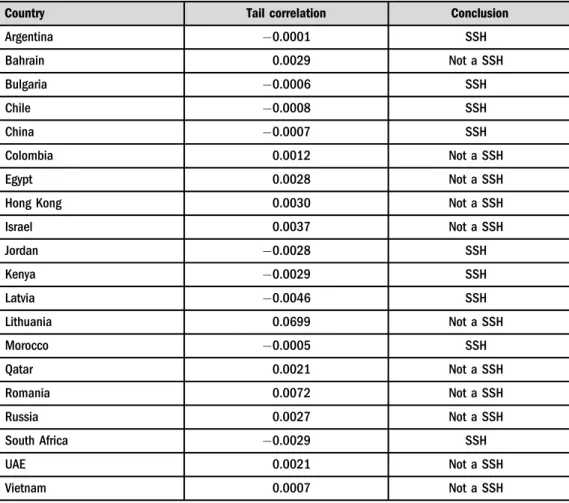
As we see inTable 4, out of 34 countries, in 20 countries gold can serve as a weak safe haven instrument. For all other countries, there is a positive probability for lower tail dependence between gold and stock market return distributions. In the next step, we estimate the tail correlation,r(X, Y|X <Xq), between stock and gold returns for those 20 countries tofind out whether gold is also a strong safe-haven instrument for the stock market portfolios in those countries. To that goal, we performed a Monte Carlo simulation to draw a sample of size 100,000,000 for each country where gold is shown as a weak SHA. These samples are drawn from the joint distribution characterized by the bestfitting copula function. Later, we calculated
Stock market returns Gold returns
Country m u a g b AIC m u a g b AIC
Argentina 0.110 0.076 0.102 0.418 0.885 4.04 0.058 0.019 0.071 0.196 0.934 3.01
(0.024) (0.016) (0.011) (0.066) (0.014) (0.013) (0.004) (0.008) (0.079) (0.007)
Bahrain 0.007 0.036 0.074 0.404 0.880 1.12 0.014 0.013 0.055 0.144 0.947 2.69
(0.01) (0.015) (0.025) (0.207) (0.039) (0.024) (0.006) (0.012) (0.189) (0.012)
Brazil 0.034 0.033 0.062 0.616 0.932 3.77 0.039 0.027 0.082 0.381 0.919 3.32
(0.022) (0.007) (0.007) (0.091) (0.008) (0.016) (0.006) (0.01) (0.081) (0.011)
Bulgaria 0.014 0.074 0.153 0.056 0.789 2.07 0.025 0.004 0.042 0.102 0.964 2.55
(0.013) (0.025) (0.03) (0.092) (0.05) (0.017) (0.002) (0.008) (0.161) (0.007)
Chile 0.044 0.035 0.122 0.305 0.865 2.43 0.043 0.010 0.048 0.312 0.955 3.07
(0.01) (0.006) (0.011) (0.051) (0.013) (0.016) (0.002) (0.005) (0.1) (0.005)
China 0.041 0.012 0.082 0.162 0.935 3.31 0.023 0.006 0.054 0.274 0.955 2.67
(0.014) (0.003) (0.009) (0.056) (0.007) (0.011) (0.001) (0.005) (0.083) (0.004)
Colombia 0.010 0.042 0.133 0.369 0.850 2.31 0.011 0.011 0.050 0.005 0.953 3.11
(0.016) (0.014) (0.026) (0.097) (0.033) (0.023) (0.005) (0.01) (0.159) (0.009)
Czech Rep. 0.046 0.026 0.118 0.286 0.886 2.97 0.018 0.010 0.052 0.333 0.952 2.80
(0.012) (0.004) (0.01) (0.048) (0.01) (0.012) (0.002) (0.006) (0.1) (0.006)
Egypt 0.113 0.063 0.131 0.184 0.859 3.55 0.022 0.021 0.068 0.263 0.934 2.84
(0.023) (0.019) (0.019) (0.069) (0.024) (0.017) (0.005) (0.009) (0.112) (0.009)
(continued)
ActaOeconomica70(2020)4,531–549
Country m u a g b AIC m u a g b AIC
Hong Kong 0.018 0.018 0.062 0.629 0.938 3.18 0.032 0.007 0.049 0.346 0.958 2.70
(0.015) (0.003) (0.006) (0.085) (0.006) (0.012) (0.001) (0.005) (0.086) (0.004)
Hungary 0.034 0.028 0.080 0.400 0.918 3.35 0.021 0.009 0.048 0.479 0.957 2.95
(0.017) (0.005) (0.008) (0.065) (0.008) (0.014) (0.002) (0.006) (0.109) (0.005)
India 0.060 0.032 0.110 0.492 0.889 3.13 0.038 0.011 0.060 0.413 0.945 2.70
(0.014) (0.005) (0.009) (0.059) (0.01) (0.012) (0.002) (0.006) (0.082) (0.006)
Indonesia 0.078 0.037 0.116 0.328 0.883 3.08 0.053 0.009 0.060 0.315 0.948 2.91
(0.013) (0.008) (0.012) (0.057) (0.013) (0.013) (0.002) (0.007) (0.085) (0.006)
Israel 0.007 0.012 0.085 0.336 0.923 2.73 0.011 0.012 0.063 0.293 0.942 2.85
(0.014) (0.004) (0.013) (0.08) (0.013) (0.016) (0.004) (0.008) (0.104) (0.008)
Jordan 0.034 0.015 0.137 0.015 0.881 1.82 0.005 0.012 0.063 0.343 0.943 2.78
(0.009) (0.004) (0.019) (0.061) (0.017) (0.017) (0.004) (0.009) (0.112) (0.008)
Kenya 0.026 0.203 0.396 0.044 0.479 2.19 0.020 0.005 0.043 0.174 0.964 2.89
(0.012) (0.03) (0.037) (0.045) (0.05) (0.016) (0.002) (0.006) (0.114) (0.005)
Latvia 0.033 0.024 0.108 0.219 0.904 2.79 0.020 0.006 0.055 0.257 0.953 2.74
(0.014) (0.007) (0.017) (0.071) (0.017) (0.013) (0.002) (0.006) (0.101) (0.005)
Lithuania 0.050 0.027 0.199 0.034 0.833 2.12 0.017 0.007 0.053 0.234 0.954 2.70
(0.007) (0.006) (0.022) (0.041) (0.02) (0.012) (0.002) (0.006) (0.098) (0.005)
(continued)
mica70(2020)4,531–549541
Stock market returns Gold returns
Country m u a g b AIC m u a g b AIC
Malaysia 0.022 0.012 0.098 0.348 0.911 1.98 0.024 0.009 0.057 0.374 0.950 2.71
(0.008) (0.002) (0.011) (0.056) (0.01) (0.012) (0.002) (0.006) (0.089) (0.005)
Mexico 0.038 0.015 0.080 0.545 0.926 2.94 0.032 0.016 0.056 0.483 0.944 3.01
(0.014) (0.003) (0.008) (0.07) (0.007) (0.014) (0.003) (0.006) (0.098) (0.006)
Morocco 0.015 0.081 0.173 0.038 0.751 2.00 0.006 0.007 0.051 0.042 0.955 2.50
(0.012) (0.02) (0.024) (0.071) (0.042) (0.016) (0.003) (0.009) (0.13) (0.008)
Peru 0.051 0.040 0.152 0.116 0.851 2.87 0.029 0.008 0.050 0.402 0.956 2.74
(0.012) (0.007) (0.015) (0.038) (0.016) (0.012) (0.002) (0.005) (0.095) (0.005)
Philippine 0.037 0.065 0.129 0.231 0.845 3.01 0.034 0.009 0.056 0.273 0.949 2.76
(0.015) (0.012) (0.013) (0.053) (0.018) (0.013) (0.002) (0.006) (0.083) (0.006)
Poland 0.041 0.016 0.070 0.319 0.932 3.01 0.008 0.013 0.058 0.459 0.945 2.90
(0.014) (0.003) (0.007) (0.064) (0.007) (0.013) (0.003) (0.007) (0.097) (0.007)
Qatar 0.073 0.103 0.275 0.190 0.726 2.62 0.007 0.010 0.058 0.244 0.949 2.82
(0.015) (0.034) (0.051) (0.072) (0.058) (0.019) (0.004) (0.009) (0.134) (0.008)
Romania 0.036 0.053 0.137 0.192 0.836 2.41 0.006 0.007 0.051 0.099 0.955 2.65
(0.016) (0.014) (0.022) (0.078) (0.029) (0.017) (0.003) (0.009) (0.137) (0.008)
Russia 0.066 0.019 0.098 0.237 0.915 3.71 0.033 0.014 0.070 0.394 0.937 2.91
(0.018) (0.004) (0.009) (0.054) (0.008) (0.013) (0.003) (0.008) (0.085) (0.007)
(continued)
ActaOeconomica70(2020)4,531–549
Country m u a g b AIC m u a g b AIC
South Africa 0.034 0.019 0.073 0.713 0.925 2.88 0.033 0.018 0.059 0.405 0.941 3.21
(0.013) (0.003) (0.008) (0.087) (0.008) (0.016) (0.004) (0.007) (0.095) (0.008)
South Korea 0.045 0.012 0.079 0.517 0.931 3.14 0.022 0.011 0.057 0.411 0.947 2.82
(0.013) (0.002) (0.008) (0.069) (0.007) (0.013) (0.002) (0.006) (0.096) (0.006)
Taiwan 0.038 0.008 0.058 0.562 0.949 3.03 0.018 0.006 0.048 0.283 0.959 2.67
(0.014) (0.002) (0.007) (0.081) (0.006) (0.011) (0.001) (0.005) (0.092) (0.004)
Thailand 0.055 0.017 0.110 0.273 0.903 2.96 0.021 0.007 0.052 0.269 0.954 2.68
(0.012) (0.004) (0.01) (0.05) (0.009) (0.011) (0.002) (0.006) (0.093) (0.005)
Turkey 0.084 0.027 0.080 0.342 0.925 3.94 0.042 0.024 0.078 0.344 0.924 3.14
(0.022) (0.006) (0.009) (0.062) (0.009) (0.014) (0.005) (0.009) (0.08) (0.01)
UAE 0.045 0.048 0.234 0.048 0.795 2.44 0.009 0.011 0.061 0.303 0.946 2.80
(0.011) (0.012) (0.03) (0.055) (0.028) (0.016) (0.004) (0.008) (0.113) (0.007)
Vietnam 0.076 0.038 0.154 0.193 0.851 3.10 0.010 0.006 0.050 0.032 0.958 2.78
(0.018) (0.009) (0.016) (0.053) (0.016) (0.016) (0.002) (0.007) (0.11) (0.005)
Notes:Table shows the TGARCH(1,1) parameter estimates for the stock market and gold returns.gis the threshold parameter to capture the assymmetric effect of positive and negative shocks. Standard errors are given in parenthesis.
mica70(2020)4,531–549543
Table 4. Bestfitting copulas
Country Best fit copula AIC λL Conclusion
Argentina BB8 306.9 0 WSH
Bahrain Joe 2662.1 0 WSH
Brazil t 31.0 þ Not a safe haven
Bulgaria Frank 2313.3 0 WSH
Chile Joe 156.3 0 WSH
China Joe 540.3 0 WSH
Colombia Frank 2395.7 0 WSH
Czech Rep. T 45.4 þ Not a safe haven
Egypt Joe 2073.5 0 WSH
HongKong Joe 273.0 0 WSH
Hungary T 59.0 þ Not a safe haven
India T 37.9 þ Not a safe haven
Indonesia T 42.7 þ Not a safe haven
Israel Frank 1283.5 0 WSH
Jordan Joe 2086.6 0 WSH
Kenya Frank 1554.7 0 WSH
Latvia Frank 508.1 0 WSH
Lithuania Gaussian 214.6 0 WSH
Malaysia T 42.9 þ Not a safe haven
Mexico T 54.8 þ Not a safe haven
Morocco Joe 2493.0 0 WSH
Peru BB7 344.5 þ Not a safe haven
Philippine T 47.1 þ Not a safe haven
Poland T 51.8 þ Not a safe haven
Qatar Joe 2669.7 0 WSH
Romania Frank 1948.1 0 WSH
Russia Joe 185.6 0 WSH
South Africa Joe 179.5 0 WSH
South Korea T 41.3 þ Not a safe haven
Taiwan T 26.4 þ Not a safe haven
Thailand T 31.8 þ Not a safe haven
Turkey T 200.5 þ Not a safe haven
UAE Joe 2168.5 0 WSH
Vietnam Joe 2128.8 0 WSH
Notes: The table shows the bestfitting copula functions for gold and equity returns. The bestfitting copula for each country is determined byfitting 39 different copula functions on the residuals constructed through TGARCH(1,1) and AIC criteria is used for best performance. WSH5Weak safe haven.
the correlation between stock and gold returns at 0.1% of stock market returns. Even though we had a very big sample size, 0.1% was the smallest percentile that yielded a stable tail correlation at each simulation.
As shown in Table 5, the tail correlation is negative only for Argentina, Bulgaria, Chile, China, Jordan, Kenya, Latvia, Morocco, and South Africa. Hence, based on our definition of strong SHAλL50 andr(X,Y|X<Xq) < 0, we reach to the conclusion that these 9 countries are the only ones in our sample where gold can act as a strong safe-haven instrument against extreme losses in the stock market.Liu (2019)looked at 16 countries in an extremal quantile regression model and he found no safe haven property of gold for all sample countries except the
Table 5.Test of strong-safe haven
Country Tail correlation Conclusion
Argentina 0.0001 SSH
Bahrain 0.0029 Not a SSH
Bulgaria 0.0006 SSH
Chile 0.0008 SSH
China 0.0007 SSH
Colombia 0.0012 Not a SSH
Egypt 0.0028 Not a SSH
Hong Kong 0.0030 Not a SSH
Israel 0.0037 Not a SSH
Jordan 0.0028 SSH
Kenya 0.0029 SSH
Latvia 0.0046 SSH
Lithuania 0.0699 Not a SSH
Morocco 0.0005 SSH
Qatar 0.0021 Not a SSH
Romania 0.0072 Not a SSH
Russia 0.0027 Not a SSH
South Africa 0.0029 SSH
UAE 0.0021 Not a SSH
Vietnam 0.0007 Not a SSH
Notes: The table shows the Monte Carlo simulation results for countries where gold is shown a weak safe haven asset. 100,000,000 samples were drawn from the joint distribution characterized by the bestfitting copula function to estimate correlation between stock and gold returns at 0.1% tail of stock returns.
SSH5Strong safe haven.
Table 6. Comparison of earlierfindings
Country Conclusion Gurgun–Unalmis (2014) Beckman et al. (2015) Baur–Dermont (2010) Chkili (2016)
Argentina SHA – – – –
Bahrain SHA Not a SHA – – –
Brazil Not a SHA SHA – SHA SHA but time-varying
Bulgaria SHA SHA – – –
Chile SHA SHA – – –
China SHA Not a SHA Not a SHA Not a SHA SHA but time-varying
Colombia SHA SHA – – –
Czech Rep. Not a SHA Not a SHA – – –
Egypt SHA Not a SHA Not a SHA – –
Hong Kong SHA – – – –
Hungary Not a SHA SHA – – –
India Not a SHA Not a SHA Not a SHA Not a SHA SHA but time-varying
Indonesia Not a SHA Not a SHA SHA – –
Israel SHA SHA – – –
Jordan SHA SHA – – –
Kenya SHA Not a SHA – – –
Latvia SHA – – – –
Lithuania SHA – – – –
Malaysia Not a SHA SHA – – –
Mexico Not a SHA SHA – – –
Morocco SHA SHA – – –
Peru Not a SHA SHA – – –
Philippine Not a SHA SHA – – –
Poland Not a SHA SHA – – –
Qatar SHA Not a SHA – – –
Romania SHA Not a SHA – – –
Russia SHA Not a SHA SHA Not a SHA SHA but time-varying
South Africa SHA Not a SHA Not a SHA – SHA but time-varying
South Korea
Not a SHA – Not a SHA – –
Taiwan Not a SHA – – – –
Thailand Not a SHA SHA Not a SHA – –
Turkey Not a SHA SHA SHA – –
UAE SHA Not a SHA – – –
Vietnam SHA Not a SHA – – –
Note: The table shows the comparison of ourfindings with the earlier ones in the literature. SHA5Strong safe haven asset.
US. He mostly look at the developed countries and there are only four countries in the sample overlapping with ours (Hungary, Russia, South Africa, and South Korea). However, our study confirms that gold serves as a weak SHA in Russia and South Africa.
We also compared our findings with the earlier ones in Table 6to make better use of the copula approach. Given the caveat that there is no consensus on the best approach to test the SHA feature and date coverage is different across studies, we looked at the overallfindings on the safe-haven feature of gold with alternative estimation methods. In a linear threshold approach,Gurgun–Unalmis (2014)found that gold serves as a safe haven for 15 of 29 sample countries. Our research can confirm theirfindings only for Bulgaria, Chile, Israel, Jordan, and Morocco. We reached to the same conclusion that gold is not a SHA for Czech Republic, India, Indonesia, Qatar, Romania, Russia, South Africa, the UAE, and Vietnam. In another study with the same econometric approach,Baur–McDermott (2010)find safe haven property of gold for Brazil. With the copula approach, wefind evidence of lower tail dependence for Brazil and reach an opposite conclusion. Chkili (2016) adopted a dynamic conditional correlation model on testing the safe haven role of gold for the BRICS countries. Our findings contradict in two countries. While he found evidence of a strong safe haven for India and Brazil during the subprime crises, our results cannot confirm it. Additionally, for Brazil, Hungary, Indonesia, Malaysia, Mexico, Peru, Philippines, Poland, Thailand, and Turkey, while other studies found evidence of safe haven role, our approach does not support that conclusion. On the other hand, for Bahrain, China, Egypt, Jordan, Kenya, Morocco, South Africa, Qatar, Romania, South Africa, the UAE, and Vietnam, we overturn the previousfindings andfind evidence for SHA role for gold in these countries. Taken all these evidence together, ourfindings can at best provide mixed findings on the safe-haven feature of gold in the sample countries.
5. CONCLUSION
Searching for a SHA, especially for the emerging and developing countries, gained more importance after the 2007 financial crisis. The literature for the advanced economies’ equity markets reaches the consensusfinding that gold is a true SHA at extreme market conditions. As for the major emerging and developing countries, thefindings are mixed. In this study, we revisit the international evidence on hedging and safe haven role of gold for 34 emerging and devel- oping countries. Given the limitations of average dependency measures at certain quantiles or the linear threshold regression models, we adopted the copula-based measure of tail dependency by modeling the joint extreme movements of gold and equity returns and tested for the safe haven property of gold both in weak and strong form. Ourfindings indicate that while gold serves as a hedge instrument for all countries in our sample, we got evidence of weak safe haven property for gold only in 20 countries. Besides, among these 20 countries only in 9 of them gold acts as a strong safe-haven instrument against extreme losses in the stock market.
Even though we find evidence of the safe-haven role of gold in more than half of our sample countries, it is difficult to generalize our findings due to the mixed evidence in our extended sample and large data span. Differences amongst the sample countries in terms of financial market depth, exporter/importer status in commodity markets, domestic markets’ correlation with developed markets, and other domestic market characteristics might play a role in this outcome. We suggest further studies to focus more on the group of markets where gold does not
serve as a SHA to see if these countries share certain characteristics when it comes to gold-stock market dynamics.
REFERENCES
Aboura, S. J.–Jammazi, R.–Tiwari, A. K. (2016): The Place of Gold in the Cross-Market Dependencies.
Studies in Nonlinear Dynamics&Econometrics, 20(5): 567–586.
Ahmed, R. R.–Vveinhardt, J. (2018): Estimation of Causal Relationship between World Gold Prices and KSE 100 Index: Evidence from Johansen Cointegration Technique.Acta Oeconomica, 68(1): 51–77.
Baur, D. G.–Lucey, B. M. (2010): Is Gold a Hedge or a Safe Haven? An Analysis of Stocks, Bonds and Gold.Financial Review, 45(2): 217–229.
Baur, D. G.–McDermott, T. K. (2010): Is Gold a Safe Haven? International Evidence.Journal of Banking&
Finance, 34(8): 1886–1898.
Beckmann, J.–Berger, T.–Czudaj, R. (2015): Does Gold Act as a Hedge or a Safe Haven for Stocks? A Smooth Transition Approach.Economic Modelling, 48: 16–24.
Bekiros, S.–Boubaker, S.–Nguyen, D. K.–Uddin, G. S. (2017): Black Swan Events and Safe Havens: The Role of Gold in Globally Integrated Emerging Markets.Journal of International Money and Finance, 73:
317–334.
Brechmann, E.–Schepsmeier, U. (2013): C-D-Vine: Modelling Dependence with C-and D-Vine Copulas in R Package CD-Vine.Journal of Statistical Software, 52(3): 1–27.
Bredin, D.–Conlon, T.–Potı, V. (2015): Does Gold Glitter in the Long-Run? Gold as a Hedge and Safe Haven Across Time and Investment Horizon.International Review of Financial Analysis, 41: 320–328.
Chkili, W. (2016): Dynamic Correlations and Hedging Effectiveness Between Gold and Stock Markets:
Evidence for BRICS Countries.Research in International Business and Finance, 38: 22–34.
Ciner, C.–Gurdgiev, C.–Lucey, B. M. (2013): Hedges and Safe Havens: An Examination of Stocks, Bonds, Gold, Oil and Exchange Rates.International Review of Financial Analysis, 29: 202–211.
Flavin, T. J.–Morley, C. E.–Panopoulou, E. (2014): Identifying Safe Haven Assets for Equity Investors through an Analysis of the Stability of Shock Transmission.Journal of International Financial Markets, Institutions and Money, 33: 137–154.
G€urg€un, G.–Unalmıs, I. (2014): Is Gold a Safe Haven Against Equity Market Investment in Emerging and Developing Countries?Finance Research Letters, 11(4): 341–348.
Hood, M. –Malik, F. (2013): Is Gold the Best Hedge and a Safe Haven Under Changing Stock Market Volatility?Review of Financial Economics, 22(2): 47–52.
Liu, W. (2019): Are Gold and Government Bond Safe-Haven Assets? An Extremal Quantile Regression Analysis.International Review of Finance, 20(2): 451–483.
Reboredo, J. C. (2013): Is Gold a Safe Haven or a Hedge for the US Dollar? Implications for Risk Man- agement.Journal of Banking&Finance, 37(8): 2665–2676.
Reboredo, J. C.–Ugolini, A. (2015): Downside/Upside Price Spillovers between Precious Metals: A Vine Copula Approach.The North American Journal of Economics and Finance, 34: 84–102.
Sklar, M. (1959):Fonctions de Repartitiona n Dimensions et Leurs Marges. Publications de l’Institut Sta- tistique de l’Universite de Paris, No. 8, pp. 229–231.
Wen, X.–Cheng, H. (2018): Which is the Safe Haven for Emerging Stock Markets, Gold or the US Dollar?
Emerging Markets Review, 35: 69–90.
Yang, L.–Hamori, S. (2014): Gold Prices and Exchange Rates: A Time-Varying Copula Analysis.Applied Financial Economics, 24(1): 41–50.
Zakoian, J. M. (1994): Threshold Heteroskedastic Models.Journal of Economic Dynamics and Control, 18(5): 931–955.