ESTIMATION OF CAUSAL RELATIONSHIP BETWEEN WORLD GOLD PRICES AND KSE 100 INDEX: EVIDENCE FROM JOHANSEN COINTEGRATION TECHNIQUE

(1)

ESTIMATION OF CAUSAL RELATIONSHIP BETWEEN WORLD GOLD PRICES

AND KSE 100 INDEX: EVIDENCE FROM JOHANSEN COINTEGRATION TECHNIQUE

Rizwan Raheem AHMED – Jolita VVEINHARDT

(Received: 11 August 2016; revision received: 10 November 2016;

accepted: 21 December 2016)

The aspiration of this research paper is to investigate the impact of international gold prices on the equity returns of Karachi Stock Index (KSE100 index) of Pakistan Stock Exchange. The daily observations from January 1, 2000 – June 30, 2016 have been divided into three sub-periods along with the full sample period on the basis of structural breaks. Descriptive analysis used to calculate the average returns, which showed signifi cant returns of KSE100 for the full sample, the fi rst and the third sample periods as compared to gold returns. Standard deviation depicted the higher volatility in all the sample periods. Correlation analysis has shown an inverse relationship amid equity returns and gold returns, whereas, Philips-Perron and Augmented Dickey-Fuller tests have been employed, and time series data became stationary after taking the fi rst difference. Johansen cointegration results have shown that the series are cointegrated in the full-sample and the fi rst sample periods.

Thus, this has demonstrated the long run association amid equity returns and gold returns in the fi rst sub-sample and the full-sample periods. However, the second and the third sub-sample periods do not exhibit long-term association amid equity returns of KSE100 and gold returns. The outcomes of Granger causality approach identifi ed bidirectional causation amid equity returns and gold returns in the full sample period in lag 2, and unidirectional causality has been observed from gold prices to stock prices in the full sample and the fi rst sub-sample periods in lag 1 and lag 2 respectively.

Keywords: Gold price, KSE 100 index, Johansen cointegration, Philips-Perron test, ADF test, Granger casualty

JEL classifi cation indices: C1, C32, E44, G14

Jolita Vveinhardt, corresponding author. Professor and Chief Researcher at the Faculty of Economics and Management, Vytautas Magnus University, Lithuania.

E-mail: Jolita.Vveinhardt@vdu.lt

Rizwan Raheem Ahmed, Professor at the Faculty of Management Sciences, Indus University,

(2)

1. INTRODUCTION

International crises, such as the oil crisis of 1973, the energy crisis in the 2000s, the global financial crises in 2008 and the Japanese asset price crises (1986–2003) had a catastrophic impact on stock markets’ investments. It brought gold in lime- light as a substitution for equity investment. It is a popular belief that investment in gold is safe in times when investment in the financial market is risky. Gold is a different kind of asset because of the inverse relation with antagonistic market shocks (Baur – McDermott 2010; Filiz et al. 2013).

Owing to numerous factors in Pakistan, gold is considered as a lucrative investment. Its recent outstanding outcome has confirmed the wit behind this con- ventional investment. Under the fluctuating market scenarios, the investors used to shift their investment from risk bearing stock investment to more secure investment in gold. Gold is often traded in dollar terms. Under uncertain conditions, investment usually flows out of budding forex markets. In Pakistan, the market volatility makes the gold investment more lucrative. The increase in gold demand has been fuelled by both depreciation in Pak Rupee (PKR) and increase in gold prices. Thus, gold is an instrumental variable and can affect the Karachi Stock Exchange 100 index (KSE100) returns in Pakistan Stock Exchange (PSX).

The excessive demand for gold in Pakistan has caused a rise in gold prices.

Apart from that, numerous other reasons are responsible for the rise in gold prices in Pakistan. Gold is considered as a secure investment. The absence of credit risk is attached to the gold investment. Even in the worst economic conditions, the liquidity of gold is established. Gold is also considered as the last resort of asset. The financial and economic systems of ancient ages and civilisations of the world demonstrates that nations have uninterruptedly expended gold as collateral versus borrowings under the struggling balance of payment stances (Shahzadi – Chohan 2010).

For centuries, the majority of the population of Pakistan and India has been using gold as an alternative source of investment. Specifically, in the South Asian region gold has been used for jewelry, helping tool in hard times, and a symbol of status.

Figure 1 depicts the trends of international gold prices and KSE100 index dur- ing the considered time period, and shows an upward trend in the international gold prices as an alternative source of investment because of the risk-free investment opportunity. Similarly, the stock prices of KSE100 index are also exceptionally well during this time period. Figure 1 also compares the trends of KSE100 index and the international gold prices during January 1, 2000 – June 30, 2016.

This research paper establishes the causal and long-term relationship between KSE100 stocks and returns to gold in the international market. It is important to

(3)

know that there is more than one element which influences the equity and gold returns. According to the investors’ point of view, these factors are alternatives to one another, responsible for price movement that are articulated as contraries in the previous literature. Specifically, gold is not considered as a local instrument of investment, but it is regarded as an international de facto commodity. Therefore, the gold prices do not only depend on local dynamics but also on the macroeconomic considerations. We have mentioned, gold prices are set in terms of the US dollar, thus, these prices are also dependent on the political and economic conditions of the World. Moreover, the crude oil prices also influence the international gold prices (Koutsoyiannis 1983; Ghosh et al. 2002; Vural 2003; Tully – Lucey 2005;Topcu 2010; Toraman et al. 2011). Similarly, the equity prices depend on numerous macroeconomic indicators, for instance, rate of inflation, exchange and interest rates, imports and exports, government debts, gold and crude oil prices, and economic growth (Fama 1981; Gong – Mariano 1997; Cheung – Lilian 1998;

Bali – Cinel 2011).

The Karachi Stock Exchange (KSE) was the oldest equity market in South Asia, and the largest one in Pakistan before the merger of the three stock markets such as KSE, Lahore stock exchange and Islamabad stock exchange. On January 11, 2016, these three markets were merged and renamed as the Pakistan Stock Exchange (PSX). As on November 17, 2017, 581 companies in 35 sec- tors are listed at PSX with total market capitalization of PKR8506.433 billions

Figure 1. Movement of gold prices (USD/Ounce) and stock price 100 index Source: Trading Economics (2016).

(4)

(USD80.249 billions). Pakistan Stock Exchange gained the status of emerging market in May 2017.

Pakistan Mercantile Exchange (PMEX) is a commodity market where gold and other commodities are being traded. PMEX is the platform for individual and institutional investors, where they trade all these commodities including gold.

The online trading services are being provided for 21 hours to the customers, PMEX is facilitating trading of gold, silver, and crude oil. There are several deals for each commodity; however, gold is traded in eight different contracts, for instance, gold 1 & 100 ounces, gold 1, 50 & 100 tola¹, gold 100 g & 1 kg, and mini-gold contracts.

The prime objective of this research is to investigate the association amid equity returns of KSE100, and changes in international gold prices. Another aim is to explore the short and/or the long run causal relations, and also the direction of causation between these variables. The daily time series data of international gold prices were taken from the official website of Trading Eonomics (2016), however, the daily data for KSE100 index were obtained from the official website of PSX. The time horizon for the undertaken study was selected from January 1, 2000 to June 30, 2016 (PSX 2016). As shown in Figure 1, there are several structural breaks during the stated time period; therefore, we have divided the data period into three sub-periods along with the full sample period as follows:

Full sample period: Janurary 1, 2000, through June 30, 2016.

First sub-sample period: January 1, 2000, through June 30, 2008.

Second sub-sample period: July 1, 2008, through June 30, 2012.

Third sub-sample period: July 1, 2012, through June 30, 2016.

The significance of this research is manyfold because very few researches have been carried out on the specific relationship between world gold prices and KSE100 returns. Most of the researches have been conducted on domestic gold price plus other macroeconomic variables in order to check the relationship with KSE100. Another distinguished aspect of our research is the data, which has been taken on a daily basis, and total 4060 observations (after adjustments) were re- corded and used for analysing the relationships of variables for all three sub- periods along with the full sample period. Secondly, the performance and growth of KSE100 index have been exceptionally well during the last few years, and it touches the 55,000 index. Hence, this exceptional growth of KSE100 index has captured the attention of foreign investors, for example, China has purchased the 40% shares of KSE100. Thus, this makes a clear differentiation for KSE100 from other regional and emerging markets and provides a substance of great relevance

1 Tola is a Hindi term which is used in India and some other Asian countries to measure gold.

At present, one tola gold is equivalent to 10 grams of gold.

(5)

and curiosity for researchers to re-investigate the characteristics of KSE100 index. This foundation has multiplied the significance of this study. Hefty devel- opments are also observed in gold prices worldwide in general and in Pakistan in particular in recent times. This has necessitated re-examining the association amid the equity returns of KSE100 index and the international gold returns. The outcomes of the undertaken research will offer valuable investment decision in- puts to the investors of the stock and gold market. Numerous research constructs are influencing the equity returns, and international gold prices happen to be an important variable. Hence the results of undertaken research are anticipated to serve an eye and ear to the stock and the gold investors.

The rest of the study is structured as follows: Section 2 overviews the relevant studies on the link among gold prices and important economic and capital markets’ variables, Section 3 comprises of the empirical framework and estimation techniques, Section 4 deals with estimations and results, whereas Section 5 con- tains the discussion and Section 6 the conclusion.

2. LITERATURE REVIEW

The findings of previous researches are hybrid; several studies are in favour of long-term relationships between changes in gold rate and equity returns. How- ever, numerous researches also concluded that gold prices and stock returns do not have any relationship in the long run.

Developed and European stock markets. According to Pritchard (2010), the global financial crises of 2008 and its transacted effects emerged as economic recession worldwide from 2008 to 2012. This economic crunch had crashed all the financial markets of the world, therefore, this catastrophe has increased the importance of gold, and investors have again diverted towards the investment opportunities in the gold market. The money and stock markets of the world have abruptly deteriorated, and consequently, money and equity markets of the world have collapsed. Hence, besides this factor, there are several other reasons, which have appreciated the demand for gold, and prices of gold have increased sharply.

Baur – Lucey (2010) explained that in some European countries like the UK, Germany, and in the USA, gold is considered as a safe mode of investment as compared to stocks. Baur – McDermott (2010) have studied both the emerging countries and the developed ones in this regard and concluded that gold is a safe heaven and hedging for US stock markets, but has not shown the same character- istic in case of Japan, Australia, Canada and BRIC countries. Bali – Cinel (2011) have studied the relationship between gold prices and equity returns of ISE in the

(6)

Turkish economy. They have used the panel analysis to examine the influence of gold prices on the equity market and also investigated the quantum and direction- ality of this effect. The results of their study demonstrated that there is no direct impact on the equity market, but the gold prices are one of the other factors which have a definite influence on the equity returns of the ISE in case of Turkey.

Sumner et al. (2010) tried to discover the mutual dependence of equity returns, bonds, and gold returns by observing the returns of gold and instabilities. As per this research, gold is just supportive in predicting stock behavioural movements.

Büyüksalvarcı (2010) studied the relationship between the equity returns, and interest rate, exchange rate, CPI, money market, oil prices, and gold prices. The results of the study have shown that the gold returns have an inverse relation to the equity returns. Omağ (2012) has investigated the association between gold prices and other macroeconomic indicators including stock prices of ISE in the Turk- ish economy. He found that the gold prices significantly influence the exchange rate and the equity returns of the ISE index. Yahyazadehfar – Babaie (2012) have shown an inverse relationship between equity returns and various economic indicators, for instance, changes in gold prices and interest rate.

Moore (1990) has demonstrated an inverse association between gold prices and stock returns. It means when stock markets deteriorate the gold prices increase or the other way round. Wang et al. (2010) have investigated the causal association between different macroeconomic indicators including gold prices, and equity returns of differnt stock markets such as Japan, Germany, Taiwan, China, and the United States, and found the long-run relationship of gold prices with equity returns except in the United States. They have used Johansen cointegration to derive the long-term causal relationship. Another study conducted by Aksoy – Topcu (2013) analysed the relationship in short and long-run changes in gold prices, equity returns, government debt securities, PPI, and CPI in Turkey.

They found an inverse relationship between equity returns and gold returns, and affirmative association amid gold price changes and PPI centered inflation rate.

Smith (2002) has investigated an association between equity returns and the changes in gold prices in both long and short run. The researcher used three different prices of gold; from the London exchange varying from 10:30 am, 15:00 pm and closing time, and for the equity returns he has considered 18 countries’

stock market indices. The results have demonstrated an inverse association between the equity returns of different markets and the gold returns in the short run, moreover, this research concluded that there is no evidence of a long-run association between the equity returns and gold returns. The findings revealed by previous research studies including Blose – Shiech (1995), Mahdavi – Zhou (1997), and Chan – Faff (1998) have demonstrated that the gold price changes are based on the inflation pressure.

(7)

South Asian stock markets. Since gold has unique values and characteristics in the South Asian countries, and it is thought that savings are risk-free in gold investment, which can be liquidated at any hard time, therefore, people prefer to save money in the shape of gold. Secondly, gold jewelry and ornaments have been considered to be the pride in these societies for centuries. Thus, the gold price has a distinguished relationship with stock returns in India, Pakistan, Bang- ladesh, Iran, etc.

Bhunia – Mukhuti (2013) have studied the influence of gold returns on equity returns of Indian stock markets (Bombay Stock Exchange & National Stock Exchange of India) and concluded that there was no causal association between changes in local gold rates and stock returns of BSE and NSE. Moreover, they have evidenced that there was no bidirectional causality between the analysed variables. Baig et al. (2013) concluded that the gold rates and prices of oil do not have any effect on the equity returns of KSE100 or the other way round. Sharma – Mahendru (2010) have examined the association amid forex rates, prices of gold, and equity returns in the Indian context and found a significant association between the variables of interest. Shahzadi – Chohan (2010) have found a negative causal association between change in gold rates and equity returns of KSE100 index. Kaliyamoorthy – Parithi (2012) researched on the link between the NSE index and the gold prices and found that no association existed between the change in gold rates and the stock index in India. However, another research has been carried out in India by Bhunia – Das (2012) which has shown a relationship between the gold rates and the returns of equities in India. They have demonstrated that the selected indicators influence each other, whereas gold prices change in cycle with equity returns during and after the global financial crunch.

Moreover, the results of the study demonstrate that the Indians have started to recognise gold not only as jewelry but also as an instrument of investment.

Mishra – Mohan (2012) studied the association between Indian financial markets and price changes in gold, and demonstrated a strongly interlinked relationship between these variables. Mishra et al. (2010) have shown a positive relation between gold prices and equity markets in India, and also confirmed that both equity returns and gold prices are essential for predicting each other. Gwilym et al. (2011) have conducted an important research on the association of equity returns and changes in gold prices and explicated the illustrative influence of gold rates with respect to future return to gold investment. Samadi et al. (2012) studied the causal relationship between inflation, gold price, oil prices, exchange rate, and equity returns of the Tehran Stock Exchange. This research determined the influence of macroeconomic indicators on equity returns from 2001 to 2010 using the GARCH model. The result brings out that a causative association held

(8)

among gold returns, interest rate, and exchange rate while no relationship lies with liquidity and price of oil.

Miscellaneous stock markets. Nguyen et al. (2012) have also tried to estab- lish the association between gold markets and equity markets. For this purpose, the market data from eight countries comprising Singapore, Japan, UK, Malay- sia, Indonesia, Philippines, Thailand and the United States were collected. This research reveals that most of the stock markets displayed unavailability of dependency with the gold price. While Kuala Lumpur equity market has right-end dependency on gold returns and Japan, Indonesia, and the Philippines markets have left-end dependency. Mulyadi – Anwar (2012) have studied the gold and stock investments, and have concluded that the gold investments are more prof- itable as compared to stocks in the equity markets of Singapore, Malaysia, and Indonesia.

Pilinkus (2009) conducted a very important study and checked the influence of 40 macroeconomic variables including gold prices on stock prices in Lithua- nian market. He has demonstrated the interrelated affect and significant influence of all macroeconomic indicators on stock prices. Lawrence (2003) determined through his study that gold is one of the most efficient diversifiers of the portfo- lio. Thus, it has no interlinks with the dynamics of macroeconomics as compared to other financial assets and a weak correlation lies between the return on gold and stocks.

3. EMPIRICAL FRAMEWORK

Descriptive analysis is used to calculate the average returns and volatility; whereas correlations analysis is used to establish the relationship between stock returns and gold returns. We have employed two stationary techniques such as Philips- Perron and Augmented Dickey-Fuller for the stationarity purposes, Johansen cointegration has been employed to examine the existence and number of cointegrating vectors, and lastly, for causality purposes, Granger test has been used.

Change in KSE100 index. KSE100 returns are computed by (1) as follows:

(1) where: SP_(t) are the returns of KSE100 index in a daytime ‘t’ and C_t & C_t–1 referred for closing and opening points of stock prices in daytimes ‘t’ & ‘t–1’, respectively.

Change in gold prices. The gold prices (GP) are calculated by (2) as follows:

( ) 1

1

t t

t

SP C C_ 

(9)

(2)

where: GP_(t) are the gold returns in daytime ‘t’, and GP_t & GP_t–1 are gold prices in the daytime, and ‘t’ & ‘t–1’ are closing and opening daytimes, respectively.

Correlation analysis. Karl Pearson Correlation analysis technique is applied to test the interconnection among the variable of interest for this study.

(3)

where: r = Correlation coefficient, x, y = Two variables’ returns and n = No. of observations.

Unit Root Tests. The initial step is to confirm the stationarity of data series, therefore, first, we check the stationarity of the data and for this purpose numerous testing methods are available but the most efficient and commonly practiced methods are Philips and Perron (1988), and Augmented Dickey-Fuller (1979, 1981). The generalised equation for Philips-Perron (PP) can be expressed in (4) as follows:

(4)

The PP test could be elaborated as the null hypothesis if p = 0, Philips-Perron (PP) has Zt & Zp statistics, which have similar asymptotic distributions as the normalized bias statistics and ADF t-statistic have possessed. The biggest advan- tage of the PP test as compared to the ADF test is that the results of PP test are more accurate and robust to overall procedures of heteroskedasticity in the white noise error ‘e_t’ term. Moreover, there is no need to stipulate a lag length in PP test for the regression test. However, ADF can be expressed in (5) as follows:

(5)

where: ‘t’ is a time period, ‘y’ is time series, ‘n’ is optimum number of lags, α₀ is known as the constant value, and ‘e’ is referred to as white noise error term.

Johansen cointegration testing approach. This approach makes the usage of cointegration between the series of similar order by creating a cointegration equation. The trend is stationary due to the constant difference between the two series, and it is feasible to describe a long-term stable relationship between the

( ) 1

1

t t

t

GP GPGP_ 

1 1 1

2 2

1 1 1 1

1

n n n

i j i j

i j i j

n n n n

i i j j

n x y x y

r

n x x n y y

   



 

   

   

   

  

   

1 .

t t t

y py e

Δ  _ 

0 1 1

1 n

t t t t

i

y α αy α y e

Δ _ Δ



  





(10)

series (Hall – Henry 1989). If cointegration is not deployed, it shows no long-run relationship between the two series (Dickey et al. 1991).

Precisely, if the time series ‘y_t’ is known as the vector for ‘n’ number of stochastic variables, subsequently there will be an existence of ‘p-lag’ vectors of auto regression besides the Gaussian errors, (6) is the mathematical form and could be written as:

(6)

In equation (6), the time series ‘y_t’ is denoted for (nx1) vectors of the considered variables, which are integrated of orders, whereas, the term ‘ε_t’ is known for (nx1) number of vectors innovations. Thus, the above (6) could be written in the form of (7) as follows:

(7)

where: ₁

1 p

i i

A

η _





^and

1

.

p

t j

j i

A τ

 





Johansen (1991, 1995), and Johansen – Juselius (1990) methods are used to classify the number of vectors for cointegration. They have devised two statistic tests in which first test is known as the Trace test or simply λ-trace in order to check the null hypothesis of a distinct number of vectors under the condition of less than or equal to the probability ‘p’ in comparison of unrestricted alternative p = r. Now, the (8) is the mathematical form of Trace test, and expressed as fol- lows:

(8)

where: ‘T’ is known as the number of utilizable observations, and the term ‘λr+1’

is known as the estimated Eigenvalue from the matrix, thus, the second test statistic is called as the Maximum Eigenvalue test or simply λ-max, and it could be estimated from (9) as follows:

(9)

The mathematical form (9) includes testing the null hypothesis of whether there is ‘r’ number of cointegrating vectors in contrast to the alternative hypothesis, which is (r+1) cointegrating vector.

Granger Causality Technique. The Granger theorem states, if two factors are cointegrated then unidirectional Granger causality must exist, and this leads towards the position in order to ascertain the relationship by the error correction model (ECM) for the confirmation of causation. The pair-wise Granger causal-

1 1 ... .

t t p t p t

y μ y y ε

Δ  Δ _  Δ _ 

1

1 1

1 n

t t t t t

i

y μ ηy τ y ε

Δ _ ^ Δ _



  





1 1

( ) ⁿ ln 1

trace r

i r

r T

λ

^Λ 

 

 

 



  

max( ,r r 1) Tln 1 _r 1 .

λ

^Λ 

 

     

(11)

ity technique helps in highlighting the causal relationship of each factor. Since we have to select lag in order to get proper results that are user-quantified. It is also noted, if data series are not stationary at I(0), and no cointegration existed amongst the factors then it is necessary to transform the series by taking first difference at I(1) and (10) would be applied (Akash et al. 2011):

(10)

where: Q_prob is called as conditional probability, ‘Φ_t’ are known as the information, which was fixed at ‘t’ time period, whereas, for the historical values ‘Wt+n’

and ‘ω_t’,are set of information, which is comprised of different values, and ‘t+n’

is known as the period of time. (10) is referred as an unlimited regression equation, which helps determine the unrestricted or unlimited residual sum of square (RSSR) and eliminate the lagged values for the selected macroeconomic indica- tor. In this method, the 1st differential is used to recognize the controlled regression in order to acquire the controlled residual sum of square (RSSR), finally integrated to order one ought to be retained the ‘0’ for entire readings of the F- statistic. The null hypothesis could be checked by using (11):

(11)

From (11), we could draw the inference that if the value of F-statistic sur- passes the critical value of the selected significance level, and p-value associated to F-Statistic is less than 0.05 then we reject the null hypothesis.

4. ESTIMATION AND RESULTS

Since there are three structural breaks in the complete sample period, i.e. from January 1, 2000 to June 30, 2016, we have estimated our results according to the following four estimation periods:

Full sample period: Jan 1, 2000 – June 30, 2016.First of all, we have estimated our results on the basis of overall data time period, however, three prominent structural breaks can be seen from Jan 1, 2000 to June 30, 2016, as depicted by Figure 1, therefore, results cannot be generalised for the whole data time period.

But first we have checked the overall impact of the variables over the full sample period, and then divided the the full period into three sub-periods according to the

( | ) ( | )

prob t n t prob t n t

Q W_ Φ Q W_ ω

0

( )

RSSR RSSUR F k k

RSSN k

  

  

 





(12)

structural breaks in order to compare the changes in sub-sample time periods with the full sample period. Thus, following are the results of the full sample period.

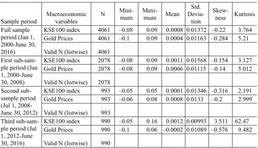
Descriptive analysis. Table 1 represents the descriptive analysis of equity re- turns of KSE100 and the daily returns of international gold prices. The descriptive statistics show that the average returns to stock for the full sample period was 0.08% per day or 24% annually, whereas, for gold prices, the average return was 0.04% per day or 12% annually. Standard deviation shows higher volatility in full sample period and almost every sub-sample period for both stock returns and gold returns. Moreover, Kurtosis values reject normality in both data series.

Total observations of 4060 were considered after adjustments.

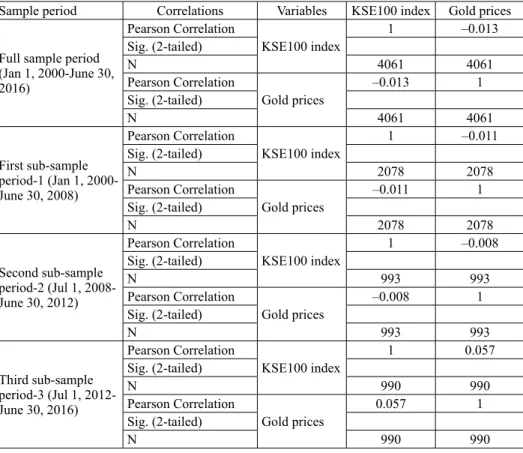
Correlation analysis. Table 2 exhibits the negative correlation between equity returns and gold returns in the full sample period thus demonstrate an inverse association between KSE100 returns and returns of gold. It is estimated from the full sample period that if stocks returns increase then gold returns decrease or the other way round. It can be concluded that the investors are very much rational about the downfall of any market, thus they switch their investments from the respective markets whenever they experience any downfall.

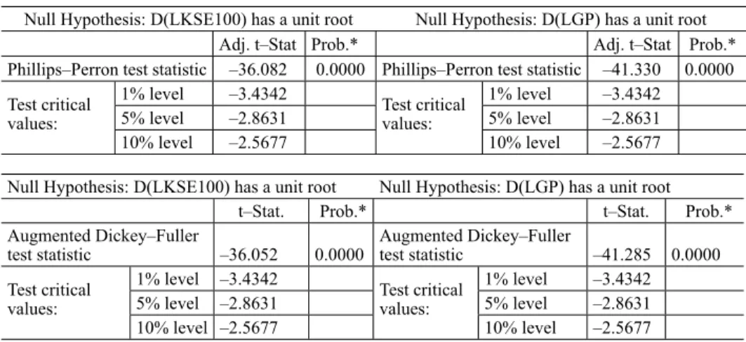
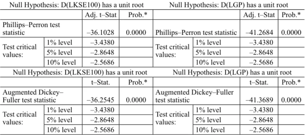
Augmented Dickey-Fuller and Philips-Perron Unit Root Tests. The out- comes of Table 3A, Table 3B, Table 3C and Table 3D indicate the findings of Philips-Perron, and Augmented Dickey-Fuller tests for the full sample period, first, second, and third sub-samples, respectively. The results of the tables show

Table 1. Descriptive analysis

Sample period

Macroeconomic variables

N Mini-

mum

Maxi-

mum Mean

Std.

Devia- tion

Skew-

ness Kurtosis Full sample

period (Jan 1, 2000-June 30, 2016)

KSE100 index 4061 –0.08 0.09 0.0008 0.01372 –0.22 3.764 Gold Prices 4061 –0.1 0.09 0.0004 0.01163 –0.284 5.21 Valid N (listwise) 4061

First sub-sample period (Jan 1, 2000-June 30, 2008)

Second sub- sample period (Jul 1, 2008- June 30, 2012)

Third sub-sample period (Jul 1, 2012-June 30, 2016)

KSE100 index 990 –0.05 0.16 0.0012 0.00993 3.511 62.47 Gold Prices 990 –0.1 0.06 –0.0002 0.01089 –0.576 9.482 Valid N (listwise) 990

Source: Own research.

(13)

that the log series of KSE100 and gold rates are non-stationary at the level form as the absolute T-statistic values are less negative as compared to the absolute critical values at 1% level of significance. Moreover, p-values associated to their corresponding T-values are greater than 0.05. Hence, it is concluded that the null hypothesis for the existence of unit root has not been rejected, thus, there is no evidence of stationarity at the level form. However, they became stationary series at the first difference because the values of absolute T-statistic are more negative as compared to the absolute critical values at 1% level of significance and corresponding p-values are less than 0.05. Therefore, the null hypothesis of the unit root has been rejected, and thus the data series of the full sample, first, second and third sub-sample periods are integrated of order one or I(1) as discussed earlier in the methodology section.

Table 2. Correlation analysis

Sample period Correlations Variables KSE100 index Gold prices

Full sample period (Jan 1, 2000-June 30, 2016)

Pearson Correlation

KSE100 index

1 –0.013

Sig. (2-tailed)

N 4061 4061

Pearson Correlation

Gold prices

–0.013 1

Sig. (2-tailed)

N 4061 4061

First sub-sample period-1 (Jan 1, 2000- June 30, 2008)

Pearson Correlation

KSE100 index

1 –0.011

Sig. (2-tailed)

N 2078 2078

Pearson Correlation

Gold prices

–0.011 1

Sig. (2-tailed)

N 2078 2078

Second sub-sample period-2 (Jul 1, 2008- June 30, 2012)

Pearson Correlation

KSE100 index

1 –0.008

Sig. (2-tailed)

N 993 993

Pearson Correlation

Gold prices

–0.008 1

Sig. (2-tailed)

N 993 993

Third sub-sample period-3 (Jul 1, 2012- June 30, 2016)

Pearson Correlation

KSE100 index

1 0.057

Sig. (2-tailed)

N 990 990

Pearson Correlation

Gold prices

0.057 1

Sig. (2-tailed)

N 990 990

(14)

Table 3A. Unit Root Tests for Stationarity Phillips-Perron & Augmented Dickey-Fuller Tests statistic

Full sample period from Jan 1, 2000 to June 30, 2016

Null Hypothesis: D(LKSE100) has a unit root Null Hypothesis: D(LGP) has a unit root

Adj. t–Stat Prob.* Adj. t–Stat Prob.*

Phillips–Perron test statistic –36.082 0.0000 Phillips–Perron test statistic –41.330 0.0000 Test critical

values:

1% level –3.4342

Test critical values:

1% level –3.4342

5% level –2.8631 5% level –2.8631

10% level –2.5677 10% level –2.5677

t–Stat. Prob.* t–Stat. Prob.*

Augmented Dickey–Fuller

test statistic –36.052 0.0000 Augmented Dickey–Fuller

test statistic –41.285 0.0000 Test critical

values:

1% level –3.4342

5% level –2.8631 5% level –2.8631

10% level –2.5677 10% level –2.5677

Note: *MacKinnon (1996) one-sided p-values.

Table 3B. Unit Root Tests for Stationarity Phillips-Perron & Augmented Dickey-Fuller Tests statistic First sub-sample period from Jan 1, 2000 to June 30, 2008

Phillips–Perron test statistic –26.7690 0.0000 Phillips–Perron test statistic –28.3688 0.0000 Test criti-

cal values:

1% level –3.4385 Test criti-

cal values:

1% level –3.4385

5% level –2.8650 5% level –2.8650

10% level –2.5687 10% level –2.5687

Augmented Dickey–Fuller

test statistic –26.7251 0.0000 Augmented Dickey–Full-er test statistic –28.3611 0.0000 Test critical

values:

1% level –3.4385 Test critical values:

1% level –3.4385

5% level –2.8650 5% level –2.8650

10% level –2.5687 10% level –2.5687

(15)

Table 3C. Unit Root Tests for Stationarity Phillips-Perron & Augmented Dickey-Fuller Tests statistic Second sub-sample period from Jul 1, 2008 to June 30, 2012

Phillips–Perron test

statistic –24.4082 0.0000 Phillips–Perron test statistic –30.369 0.0000 Test critical

values:

1% level –3.4380

5% level –2.8648 5% level –2.8648

10% level –2.5686 10% level –2.5686

Augmented Dickey–Full-

er test statistic –24.3744 0.0000 Augmented Dickey–Fuller

values:

1% level –3.4380

5% level –2.8648 5% level –2.8648

10% level –2.5687 10% level –2.5687

Table 3D. Unit Root Tests for Stationarity Phillips-Perron & Augmented Dickey-Fuller Tests statistic

Third sub-sample from Jul 1, 2012 to June 30, 2016

Phillips–Perron test

statistic –36.1028 0.0000 Phillips–Perron test statistic –41.2684 0.0000 Test critical

values:

1% level –3.4380

5% level –2.8648 5% level –2.8648

10% level –2.5686 10% level –2.5686

Augmented Dickey–

Fuller test statistic –36.2545 0.0000 Augmented Dickey–Fuller

values:

1% level –3.4380

5% level –2.8648 5% level –2.8648

10% level –2.5686 10% level –2.5686

(16)

VAR Lag Order Estimation. As stock returns data series has become station- ary at first difference, and the data series of gold returns is also integrated of order one, therefore, the Johansen cointegration test is suggested. In order to find out the appropriate lag length, we employed the lag length selection criteria that fol- lowed the Akaike (1973) information criterion (AIC). The AIC has proposed 2 lags for all data series in first, second, and third sub-sample periods, and the full sample period as well.

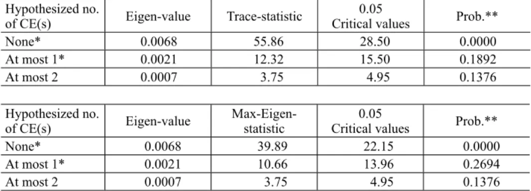
Johansen Cointegration Test Results. This test is applied to find out if cointe- gration exists and also to determine the figure of cointegration relation, whether it is long-term between equity returns and gold returns. The results in Table 4, for the full sample period, showed a long-term association between equity returns and gold returns. The outcomes of Table 4 further indicate that both variables are cointegrated because both approaches such as Trace test and Max-Eigen-value test have rejected the null hypothesis of no cointegration. Thus, it has further confirmed the existence of 2 significant cointegrating vectors that demonstrated 2 common stochastic trends in the model, and this is also an evidence of market cointegration. Hence, it indicates existence of stationarity and confirmed the long run relationship between equity returns of KSE100 and returns of gold.

Results of Granger Causality Technique. We have employed a pair-wise Granger causality technique that helps in highlighting the causal relationship between each factor. Since we have to select a lag in order to get proper results that is user-counted to check the sessions calculation. Table 5 shows that there is a

Table 4. Johansen Cointegration Test Result (Trace & Max-Eigenvalue) Unrestricted Cointegration Rank Test (Trace & Max-Eigenvalues)

Full sample period from Jan 1, 2000 to June 30, 2016 Hypothesized no.

of CE(s) Eigen-value Trace-statistic 0.05

Critical values Prob.**

None* 0.0068 55.86 28.50 0.0000

At most 1* 0.0021 12.32 15.50 0.1892

At most 2 0.0007 3.75 4.95 0.1376

Hypothesized no.

of CE(s) Eigen-value Max-Eigen-

statistic 0.05

Critical values Prob.**

None* 0.0068 39.89 22.15 0.0000

At most 1* 0.0021 10.66 13.96 0.2694

At most 2 0.0007 3.75 4.95 0.1376

Notes: Both Trace & Max-Eigenvalue Tests signify 2 cointegrating equ(s) at 0.05 levels. * indicates rejection of null hypothesis at 0.05 significance level, ** MacKinnon-Haug-Michelis (1999) p-values. Lags interval (in first difference): 1 to 4.

(17)

unidirectional causality from gold prices to KSE100 index in lag 1, but bi-direc- tional causality existed between KSE 100 index and gold price in lag 2. It is also important to comprehend that even if there is a causality among the variables, it does not evidence the movement of one variable due to the movement of another variable. It is well known, to a certain degree that causality fundamentally is una- voidable for the movements in time series (Awe 2012).

First sub-sample period: Jan 1, 2000 – June 30, 2008. Table 1 shows that in the first sub-sample period, the average stock returns were 0.11% daily or 33%

annually, while the gold returns were 0.06% daily or 18% annually. It shows that the average stock returns are significantly much higher in the first sub-sample period than in comparison to the full sample period. Moreover, the stock returns are also much higher than the gold returns in the first sample period. Standard deviation shows the higher volatility in this sample period for both stock returns and gold returns too. Moreover, Kurtosis values again reject normality in both data series. Total observations of 2078 were considered after adjustments.

Correlation analysis. The outcomes of Table 2 exhibit negative correlation between equity returns and gold returns in the first sub-sample period that demonstrates an inverse association between KSE100 returns and returns of gold.

Thus, this is the evidence that investors divert their investments from stock market to gold in the declining period or the other way round.

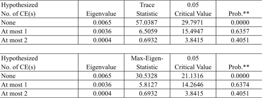
Johansen Cointegration Test Results. The results of Table 6 for the first sub-sample period, showed a long-term association between equity returns and gold returns. The outcomes of Table 6 further indicate that both variables are

Table 5. Pair-wise Granger Causality Tests Full sample period from Jan 1, 2000 to June 30, 2016 Lags: 1

Null Hypothesis: Obs. F-Statistic Prob. Decision

DLGP does not Granger Cause

DLKSE100 4060 4.84254 0.0120 Reject Ho

DLKSE100 does not Granger

Cause DLGP 2.17974 0.2517 Does not reject Ho

Lags: 2

DLKSE100 4060 5.13855 0.0311 Reject Ho

Cause DLGP 2.06664 0.0525 Reject Ho

(18)

cointegrated because both approaches such as Trace test and Max-Eigen-value test have rejected the null hypothesis of no cointegration. Thus, it has further confirmed the existence of 1 significant cointegrating vector that demonstrated 1 common stochastic trend in the model, and this is also an evidence of market cointegration. Hence, it indicates an existence of stationarity and confirmed the long run relationship between equity returns of KSE100 and returns to gold in the first sub-sample period.

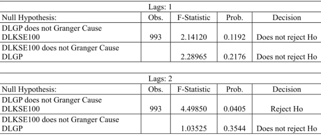
Results of Granger Causality Technique. It is confirmed from Table 7 that there was no causality between KSE100 stock returns and gold returns in either direction in lag 1, but unidirectional causality existed between KSE100 index and gold price in lag 2 from gold prices to equity prices in the first sub-sample period.

Second sub-sample period: July1, 2008 – June 30, 2012. The global finan- cial crises had started in 2008 and eventually converted into global economic recession from 2008 to 2012. Every financial market of the World had crashed in 2008, faced a deep financial crisis and had shown a declining trend in this period.

Figure 1 also shows a structural break and continuous declining in KSE100 index during this time frame. Thus, considering the second sub-sample period, we ad- dress this problem when KSE100 index was declining, but intense and continuous investments were made in gold prices during that period. The results of our

First sub-sample period from Jan 1, 2000 to June 30, 2008

Hypothesized Trace 0.05

No. of CE(s) Eigenvalue Statistic Critical Value Prob.**

None 0.0065 57.0387 29.7971 0.0000

At most 1 0.0036 6.5059 15.4947 0.6357

At most 2 0.0004 0.6932 3.8415 0.4051

Hypothesized Max-Eigen- 0.05

No. of CE(s) Eigenvalue Statistic Critical Value Prob.**

None 0.0065 30.5328 21.1316 0.0000

At most 1 0.0036 5.8127 14.2646 0.6374

At most 2 0.0004 0.6932 3.8415 0.4051

(19)

research also proved the deteriorating behavior of KSE100 index and its impact on gold prices as follows:

Descriptive analysis. Table 1 shows that the results of returns were entirely different as compared to the previously discussed first sub-period, stock returns show daily 0.01% returns or annually 3%, whereas, daily gold returns were 0.08%

or 24% annually. It shows that the average gold returns are much higher as compared to the previous sub-periods, and it is also noted that the gold returns are significantly higher than the stock returns in the second sample period. Thus, these results proved that gold was gaining the utmost attention of local and international investors and they diverted their investment from stock market to gold market in Pakistan. Standard deviation shows higher volatility in this sample period for both equity returns and returns of gold. The outcomes of the second sub-period confirmed the trend of Gold prices & KSE100 when the second structural break has taken place and gold prices surpass the stock returns. Total observations of 993 were taken after adjustments for the second sub-period.

Correlation analysis. The outcomes of Table 2 again exhibit negative correla- tion between equity returns and gold returns in the second sub-sample period that demonstrates an inverse association between KSE100 returns and returns of gold.

Thus, this is the evidence that investors divert their investments from stock market to gold in the declining period specifically for the second sub-sample period.

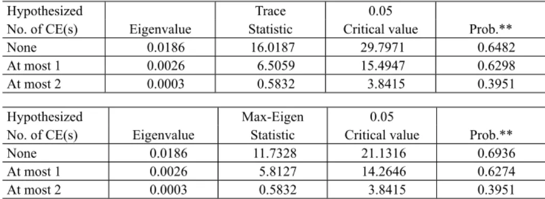
Johansen Cointegration Test Results. The results of Table 8, for the second sub-sample period, show no existence of the long-term association between equity returns and gold returns. Table 8 further indicates that both variables are not cointegrated because both approaches such as Trace test and Max-Eigen-value

Table 7. Pairwise Granger Causality Tests First sub-sample period from Jan 1, 2000 to June 30, 2008

Lags: 1

DLKSE100 993 2.14120 0.1192 Does not reject Ho

DLKSE100 does not Granger Cause

DLGP 2.28965 0.2176 Does not reject Ho

Lags: 2

DLKSE100 993 4.49850 0.0405 Reject Ho

DLKSE100 does not Granger Cause

DLGP 1.03525 0.3544 Does not reject Ho

(20)

test have not rejected the null hypothesis of no cointegration. Thus, it is further confirmed that there is no existence of cointegrating vector in the model. Hence, it indicates that there is no long-run relationship between equity returns of KSE100 and returns of gold in the second sub-sample period.

Results of Granger Causality Technique. We have employed a pair-wise Granger causality technique that helps in highlighting the causal relationship between each factor. Since we have to select a lag in order to get proper results that is user-counted to check the sessions calculation. Table 9 shows that there is no

Second sub-sample period from Jul 1, 2008 to June 30, 2012

Hypothesized Trace 0.05

No. of CE(s) Eigenvalue Statistic Critical value Prob.**

None 0.0186 16.0187 29.7971 0.6482

At most 1 0.0026 6.5059 15.4947 0.6298

At most 2 0.0003 0.5832 3.8415 0.3951

Hypothesized Max-Eigen 0.05

No. of CE(s) Eigenvalue Statistic Critical value Prob.**

None 0.0186 11.7328 21.1316 0.6936

At most 1 0.0026 5.8127 14.2646 0.6274

At most 2 0.0003 0.5832 3.8415 0.3951

Table 9. Pairwise Granger Causality Tests

Second sub-sample period from Jul 1, 2008 to June 30, 2012 Lags: 1

Lags: 2

(21)

causality between KSE100 stock returns and gold returns in either direction in lag 1. Similarly, in lag 2 there is no evidence of any causality in either direction, thus, it implies that in the second sub-sample period no variables Granger cause another.

Third sub-sample period: July 1, 2012 – June 30, 2016. After the financial crises, investors moved into the precious metal market, and investors diverted their investments in gold. Figure 1 shows evidence that there was a continuous increase in international gold prices during the period from 2008 to 2011 and prices peaked in 2011. But at the end of 2011, there was a continuous decline in gold prices. So, this was the third structural break in our data due to regular decline in gold prices, but at the same time KSE100 index was recovering and gaining momentum. Therefore, the third sub-sample period is very important to establish the relationship between stock returns and gold returns when both variables get apart and swinging towards different poles. The results of our study for this period also demonstrated comprehensively for this phenomenon.

Descriptive analysis. Table 1 represents the descriptive analysis of equity re- turns of KSE100 and the daily returns of international gold prices. The results of Figure 1 and Table 1 clearly demonstrated that there is another structural break in data time series because the stock returns suddenly rise and reach the level of 0.12% daily or 36% annual returns, but at the same time there is a sharp decline in gold returns and it becomes negative i.e. –0.02% daily or –6% annual returns.

These results are very much on similar line with the international financial markets as happened in Pakistan when investors again moved into KSE100 stock market because of declining returns to gold. Standard deviation again shows the higher volatility in the third sub-sample period for both stock returns and gold returns. Total observations of 990 were considered after adjustments.

Correlation analysis. The outcomes of Table 2 strikingly show the positive but insignificant correlation between equity returns and gold returns in the third sub- sample period that demonstrates a direct association between KSE100 returns and returns of gold. It is further concluded that the gold prices and the stock prices move together but yield a difference, which clearly indicates that the investors are in favor of stock returns rather than gold returns during the third sub-sample period.

Johansen Cointegration Test Results. The results of Table 10, for the third sub-sample period, show no existence of a long-term association between equity returns and gold returns. Table 10 further indicates that both variables are not cointegrated because both approaches such as Trace test and Max-Eigen-value test have not rejected the null hypothesis of no cointegration. Thus, it is further confirmed that there is no existence of cointegrating vector in the model.

Hence, it is implied that there is no long-run relationship between equity returns of KSE100 and returns of gold in the third sub-sample period. Figure 1 also

(22)

depicts that there is a structural break and both data time series are getting apart in this period and the outcomes of Johansen cointegration also substantiated the existence of no long-term association in the third sub-sample period.

Results of Granger Causality Technique. We have employed a pair-wise Granger causality technique that helps in highlighting the causal relationship between each factor. Since we have to select a lag in order to get proper results that is user-counted to check the sessions calculation. Table 11 shows that there is no

Third sub-sample period from Jul 1, 2012 to June 30, 2016

Hypothesized Trace- 0.05

No. of CE(s) Eigen-value Statistic Critical value Prob.**

None 0.0898 15.6781 29.7971 0.7871

At most 1 0.0336 5.9843 14.2646 0.7210

At most 2 0.0005 1.8856 3.8415 0.1610

Hypothesized Max-Eigen- 0.05

No. of CE(s) Eigen-value Statistic Critical value Prob.**

None 0.0885 12.4560 21.1316 0.7698

At most 1 0.0335 5.8890 14.2646 0.7122

At most 2 0.0005 1.8965 3.8415 0.1638

Table 11.Pairwise Granger Causality Tests Third sub-sample period from Jul 1, 2012 to June 30, 2016