Properties of risk capital allocation methods: Core Compatibility, Equal Treatment Property and Strong
Monotonicity
by Dóra Balog, Tamás László Bátyi, Csóka Péter, Miklós Pintér
C O R VI N U S E C O N O M IC S W O R K IN G P A PE R S
CEWP 13 /2014
Properties of risk capital allocation methods:
Core Compatibility, Equal Treatment Property and Strong Monotonicity ∗
D´ ora Balog
†, Tam´ as L´ aszl´ o B´ atyi
‡,
P´ eter Cs´ oka
§and Mikl´ os Pint´ er
¶July 23, 2014
Abstract
In finance risk capital allocation raises important questions both from theoretical and practical points of view. How to share risk of a portfolio among its subportfolios? How to reserve capital in order to hedge existing risk and how to assign this to different business units?
We use an axiomatic approach to examine risk capital allocation, that is we call for fundamental properties of the methods. Our start- ing point is Cs´oka and Pint´er (2011) who show by generalizing Young (1985)’s axiomatization of the Shapley value that the requirements of Core Compatibility, Equal Treatment Property and Strong Mono- tonicity are irreconcilable given that risk is quantified by a coherent measure of risk.
In this paper we look at these requirements using analytic and simulations tools. We examine allocation methods used in practice
∗P´eter Cs´oka thanks funding from HAS (LP-004/2010) and OTKA (PD 105859). Mik- l´os Pint´er acknowledges the support by the J´anos Bolyai Research Scholarship of the Hungarian Academy of Sciences and OTKA (K 101224).
†Corvinus University of Budapest, Department of Finance.
‡University of California, Berkeley, Department of Economics.
§Department of Finance, Corvinus University of Budapest and “Momentum” Game Theory Research Group, Centre for Economic and Regional Studies, Hungarian Academy of Sciences. E-mail: peter.csoka@uni-corvinus.hu.
¶Corvinus University of Budapest, Department of Mathematics and MTA-BCE “Len- d¨ulet” Strategic Interactions Research Group. E-mail: miklos.pinter@uni-corvinus.hu.
and also ones which are theoretically interesting. Our main result is that the problem raised by Cs´oka and Pint´er (2011) is indeed relevant in practical applications, that is it is not only a theoretical problem.
We also believe that through the characterizations of the examined methods our paper can serve as a useful guide for practitioners.
Keywords: Coherent Measures of Risk, Risk Capital Allocation, Shapley value, Core, Simulation
JEL Classification: C71, G10.
1 Introduction
Proper measurement of risk is essential for banks, insurance companies, port- folio managers and other units exposed to financial risk. In this paper we consider the class of coherent measures of risk 1 (Artzner, Delbaen, Eber, and Heath, 1999), which are defined by four natural axioms: Monotonicity, Translation Invariance, Positive Homogeneity and Subadditivity. Coherent measures of risk are broadly accepted in the literature, for a further theo- retical foundation of the notion see Cs´oka, Herings, and K´oczy (2007) and Acerbi and Scandolo (2008).
Subadditivity captures the notion of diversification: if a financial unit (portfolio) consists of more subunits (subportfolios), then the sum of the risks of the subunits is at least as much as the risk of the main unit. The risk of the main unit should be allocated to the subunits (resulting in risk savings) using a risk allocation method. This process is called risk capital allocation and has the following applications (see for instance Denault (2001);
Kalkbrener (2005); Valdez and Chernih (2003); Buch and Dorfleitner (2008);
Homburg and Scherpereel (2008); Kim and Hardy (2009); Cs´oka, Herings, and K´oczy (2009)):
1. financial institutions divide their capital reserves among business units, 2. strategic decision making regarding new business lines,
3. product pricing,
4. (individual) performance measurement, 5. forming risk limits,
6. risk sharing among insurance companies.
1As a further reading on risk measures we suggest Krokhmala, Zabarankin, and Uryasev (2011).
The Shapley value Shapley (1953) is a well established method in coop- erative game theory for allocating gains and costs. By generalizing Young (1985)’s axiomatization of the Shapley value Cs´oka and Pint´er (2011) show that when using any coherent measure of risk there is no risk capital alloca- tion method satisfying three fairness requirements at the same time: Core Compatibility, Equal Treatment Property and Strong Monotonicity. The description of the properties is as follows.
Core Compatibility ensures that the risk of the main unit is allocated in such a way that no subset (coalition) of subunits is allocated more risk capital than it would be implied by its own risk. Otherwise the given subunit coalition would strongly argue against the allocation and block it, or at least think that it is not fair. Core Compatibility means that the allocation is in the core of the resulting cooperative game. Equal Treatment Property requires that subunits having the very same risk contributions (alone and also when joining to any subset of other subunits) are treated in the same way, that is the same risk capital is allocated to each of them. It is even possible that applying a method not satisfying Equal Treatment Property might have legal consequences. Strong Monotonicity requires that if a subunit weakly reduces its stand-alone risk and also its risk contribution to all the subsets of the other subunits, then its allocated capital should not increase. This way weakly better relative performance is weakly rewarded, thus the subunits are not motivated to increase their risk.
As there is no risk capital allocation method that satisfies all the above given properties at the same time when risk is calculated by a coherent mea- sure of risk, we analyze seven allocation methods to find out how they are related to the three fairness requirements. The seven methods are: Activity based method (Hamlen, Hamlen, and Tschirthart (1977)), Beta method (see for instance Homburg and Scherpereel (2008)), Incremental method (see for instance Jorion (2007)), Cost gap method (Driessen and Tijs (1986)), Eu- ler method (see for instance Buch and Dorfleitner (2008)), Shapley method (Shapley, 1953) and the Nucleolus method (Schmeidler, 1969).
We use two different approaches. First, we discuss analytically which properties are met by the different methods. Our results are as follows: from the seven methods, two methods, well-known from game theory, the Shapley and the Nucleolus methods show the best performance, as both of them satisfy two of the three properties. In case of the Shapley method we have to give up Core Compatibility, while Strong Monotonicity is not met by the Nucleolus method. Then, we analyze Core Compatibility for all the methods using simulations. We examine how often it is fulfilled for normal and also for fat tailed (see for instance (Cont, 2001)) return distributions. Our results are presented in the tables of Section 4.
Since Cs´oka and Pint´er (2011) show that for risk capital allocation sit- uations the only allocation method satisfying Equal Treatment Property, Strong Monotonicity and Efficiency (allocating all the risk of the main unit) is the Shapley method, violation of Core Compatibility in case of the Shapley method calls for special attention. Our simulations results show that Core Compatibility is violated by the Shapley method in a significant number of the cases in every examined simulation setting. Hence we conclude that the theoretical problem raised by Cs´oka and Pint´er (2011), the impossibil- ity of the existence of an ideal risk capital allocation method, is not only theoretically important, but it is also a relevant practical problem. Thus all of the examined methods have their own advantages and disadvantages.
Practitioners have to decide on the applied method in each single situation, considering which method fits best the actual setting. Our analytical and simulation results are intended to help in this decision.
The setup of our paper is as follows: in the next section we define the notions used in our analysis. In Section 3 we introduce the seven examined methods, while we present our results in the last section.
2 Preliminaries
In this paper, for the sake of simplicity, we will assume that the subunits can be described by random variables defined on a finite probability field (Ω,M, P). We will denote random variables as X : Ω → R. As we have a finite number of states, we can think of the random variables as vectors (their components are the elements of Ω). The set of the random variables defined on the fixed finite probability field (Ω,M, P) is denoted by X.
We analyze the following financial situation. A financial unit (for instance a bank, a portfolio, etc.) consists of a finite number of subunits. The set of the subunits are denoted by N ={1,2, . . . , n}. Every financial unit can be described using a random variable, for subuniti it is random variableXi. In other words, the vector Xi shows the possible profits of subunit ifor a given time period (negative values mean losses). We are also interested in subsets of subunits, a coalition S ⊆ N is described by XS = P
i∈SXi, where the value of the empty sum is the 0 function (vector).
The function ρ : X → R is called a measure of risk. A measure of risk assigns a number to every random variable, it defines the risk of every coalition. This notion of risk can also be taken as the minimum level of capital (cash) to be added to the portfolio. In this paper we restrict ourselves to coherent measures of risk (Artzner et al, 1999). In our simulations we use the k%-Expected Shortfall measure of risk (Acerbi and Tasche, 2002), which
is the average of the worst k percentage of the losses. At last, the notion risk capital allocation situation, RCAS is used for the vectors describing the financial subunits and the measure of risk together, soXNρ ={N,{Xi}i∈N, ρ}
is a risk capital allocation situation. The class of risk capital allocation situations with the set of subunits N will be denoted by RCASN.
Example 2.1. Consider risk capital allocation situation XNρ where set Ω = {ω1, ω2, ω3, ω4}, M denotes all subsets of Ω and P is such that P({ω1}) = P({ω2}) =P({ω3}) =P({ω4}) = 14. We have three subunits, N ={1,2,3}, and the applied measure of risk ρ is the 25%-Expected Shortfall, which in this case (and for all k ∈ [0,25]) equals the maximum loss. The vectors Xi are shown in the following Table 1.
Ω/XS X1 X2 X3 X{1,2} X{1,3} X{2,3} X{1,2,3}
ω1 −10 −10 0 −20 −10 −10 −20 ω2 −3 −4 −100 −7 −103 −104 −107 ω3 −6 0 −99 −6 −105 −99 −105 ω4 0 −6 −99 −6 −99 −105 −105 ρ(XS) 10 10 100 20 105 105 107
Table 1: The risk capital allocation situation XNρ
The lowermost row contains the risk of each coalition. Note that a sig- nificant diversification effect arises when the three subunits form a coalition:
ρ(XN) = 107<120 =X
i∈N
ρ(Xi).
As in the above example, two questions arise in most of the risk capital allocation situations. How to allocate the diversification benefits among the subunits? What properties should the applied allocation method have?
The function ϕ : RCASN → RN is called risk capital allocation method (allocation method for short). A risk capital allocation method determines the allocated risk for each subunit in the particular risk capital allocation situation. We define three properties of allocation methods.
Definition 2.2. The risk capital allocation method ϕ satisfies
1. Core Compatibility (Core Compatibility) if for each risk capital alloca- tion situation XNρ ∈RCASN the equalityρ(XN) =P
i∈Nϕi(XNρ)holds, and for all coalition S ⊂N we have that ρ(XS)≥P
i∈Sϕi(XNρ),
2. Equal Treatment Property if for all risk capital allocation situation XNρ ∈RCASN and subunits i, j ∈N the equations ρ(XS∪{i})−ρ(XS) = ρ(XS∪{j})−ρ(XS), S⊆N \ {i, j} imply thatϕi(XNρ) =ϕj(XNρ),
3. Strong Monotonicity if for all risk capital allocation situationsXNρ1, YNρ2 ∈ RCASN and subunit i ∈ N the inequalities ρ1(XS∪{i})− ρ1(XS) ≤ ρ2(YS∪{i})−ρ2(YS), S⊆N imply thatϕi(XNρ)≤ϕi(YN%).
The properties can be explained as follows. Core Compatibility is satisfied if a risk allocation is stable: the risk of the main unit is fully allocated and no coalitions of the subunits would like to object their allocated risk capital by saying that their risk is less than the sum of the risks allocated to the members of the particular coalition. Equal Treatment Property makes sure that equivalent subunits are treated equally, that is if two subunits make the same risk contribution to all coalitions not containing them (also to the empty set, meaning that their stand-alone risks are the same), then the rule should allocate the very same risk capital to the two subunits. Strong Monotonicity requires that if the contribution of risk of a subunit to all the coalitions of subunits is not decreasing, then its allocated risk capital should not decrease either. Hence, as an incentive compatibility notion, the subunits are not motivated to increase their contribution of risk.
Then, the following theorem holds.
Theorem 2.3(Cs´oka and Pint´er (2011)). Considering risk capital allocation situations with coherent measures of risk there is no risk capital allocation method meeting the conditions of Core Compatibility, Equal Treatment Prop- erty and Strong Monotonicity at the same time.
Next, we look at different methods and check which property they violate.
The main goal of this paper is to find out how relevant this problem is in practice, considering return distributions having empirically observable characteristics. This question is answered in Section 4.
3 Risk capital allocation methods
In this section we present the seven risk capital allocation methods that we examine in this paper. In case of the first four methods we follow Homburg and Scherpereel (2008). The fifth method, the Euler method has different versions, we take the most “general” one. The last two methods, the Shapley (Shapley, 1953) and the Nucleolus method (Schmeidler, 1969) are well-known in game theory.
3.1 Activity based method
The method was first introduced by Hamlen et al (1977). It allocates the joint risk to the subunits in proportion to their own risk. For a risk capital allocation situation XNρ ∈ RCASN and subunit i ∈ N the Activity based method allocates
ϕABi (XNρ) = ρ(Xi) P
j∈N
ρ(Xj)ρ(XN) .
A really serious drawback of the method is that it does not consider the dependence structure of the subunits, that is it does not allocate smaller risk capital to those subunits that are hedging the others.
3.2 Beta method
LetXNρ ∈RCASN be a risk capital allocation situation and let Cov(Xi, XN) denote the covariance between the random variables describing the financial position of subunit i∈N and the main financial unit. Let the beta of unit i beβi = Cov(XCov(Xi,XN)
N,XN). Then for a risk capital allocation situationXNρ ∈RCASN and subunit i∈N the Beta method allocates
ϕBi (XNρ) = βi P
j∈N
βjρ(XN).
We have to mention that the Beta method is not always defined. If for instance the realization vector of the main unit has the same elements in all states of nature, then all of the betas are zeros, so the above given formula can not be applied.
3.3 Incremental method
The Incremental method (see for instance Jorion (2007)) defines the risk capital allocated to a subunit in proportion to its individual “risk increment”, which is its contribution of risk to the main unit. For a risk capital allocation situationXNρ ∈RCASN and subuniti∈N the Incremental method allocates
ϕNi (XNρ) = ρ(XN)−ρ(XN\{i}) P
j∈N
ρ(XN)−ρ(XN\{j})ρ(XN) .
We also have to mention that this method is not always defined, for example when we consider the risk capital allocation situation generated by
the identity matrix multiplied by minus one, then for each subunit iwe have ρ(XN)−ρ(XN\{i}) = 0, so the above given formula can not be applied.
3.4 Cost gap method
After a smaller amendment of the Incremental method, we get the Cost gap allocation rule introduced by Driessen and Tijs (1986). First of all, let us define for each subunit i∈N its smallest cost gap γi as follows:
γi = min
S⊆N, i∈S
ρ(XS)−X
j∈S
(ρ(XN)−ρ(XN\{j}))
.
The term behind the minimum operator is the cost gap of coalition S, showing the difference between the risk of the coalition and the sum of the risk contributions of its members to the grand coalition; it is in fact the non- separable risk (cost) of coalition S. By modifying the Incremental method in such a way that the non-separable risk of the grand coalition is shared proportionally to the cost gap of each player, we get the Cost gap method.
Formally, for a risk capital allocation situation XNρ ∈ RCASN and subunit i∈N the Cost gap method is defined as follows: If P
j∈N
γj = 0, then ϕCGi (XNρ) =ρ(XN)−ρ(XN\{i}),
otherwise
ϕCGi (XNρ) =ρ(XN)−ρ(XN\{i}) + γi
P
j∈N
γj ρ(XN)−X
j∈N
(ρ(XN)−ρ(XN\{j}))
! .
3.5 Euler method
The Euler method, also called gradient method or marginal contribution to risk, is a popular method both in the literature and in practice. Despite its popularity, the method is not canonically defined, that is, different versions of the Euler method are used in the literature. In this paper we introduce a notion of Euler method which is quite general, and reflects the main intuitions behind the method.
For a risk capital allocation situation XNρ ∈ RCASN and subunit i ∈ N we define the Euler method as it allocates
ϕEi (XNρ) = ρ0(XN, Xi) ,
whereρ0(XN, Xi) is the directional derivative ofρatXN alongXi. In case of the directional derivative of ρ at XN exists along each Xi, i ∈N, the Euler method is defined.
In some papers the Euler method is used in a different, more restric- tive way. The derivatives are not directional derivatives, but partial deriva- tives. In this case for any risk capital allocation situation XNρ ∈ RCASN and subunit i ∈ N the allocated risk by the Euler method is the following:
ϕEi (XNρ) =ρ0i(XN), where ρ0i(XN) is the partial derivative of the measure of risk ρ atXN along Xi.
Notice that, if for all i ∈ N the measure of risk ρ is directionally dif- ferentiable at XN along both Xi and −Xi, then ρ0i(XN) is defined. Buch and Dorfleitner (2008) show that in this case the Euler method satisfies Core Compatibility. However, many coherent measures of risk fail to meet this differentiability condition, for instance (as we will show it in Example 4.5) in general the Expected Shortfall does not meet this condition.
Moreover, by the partial derivative definition the Euler method coincides with the Aumann-Shapley value (Aumann and Shapley, 1974), and it can be extended to cases where it is not defined, in a way that it preserves Core Compatibility (Boonen, De Waegenaere and Norde, 2012); of course this extension differs from the one (directional derivative) we use in this paper.
3.6 Shapley method
The Shapley method (Shapley, 1953) gives the risk capital allocated to the subunits as follows: for a risk capital allocation situation XNρ ∈RCASN and subunit i∈N
ϕShi (XNρ) = X
S⊆N\{i}
|S|!(|N| − |S| −1|)!
|N|! (ρ(XS∪{i})−ρ(XS)), where |S| denotes the number of elements ofS.
3.7 Nucleolus method
The Nucleolus method (Schmeidler, 1969) defines the risk capital allocated to the subunits as follows: for a risk capital allocation situation XNρ ∈RCASN and subunit i∈N
ϕN ci (XNρ) = {x∈I(XNρ) :E(x)≥lexE(y) for all y∈I(XNρ)} , where I(XNρ) = {x ∈ RN : P
j∈Nxj = ρ(XN) and for all j ∈ N, xj ≤ ρ(Xj)}, E(x) = (· · · ≥ ρ(XS)−P
i∈Sxi ≥ · · ·)S⊂N, and ≥lex denotes the lexicographic ordering.
We conclude this section with the continuation of Example 2.1.
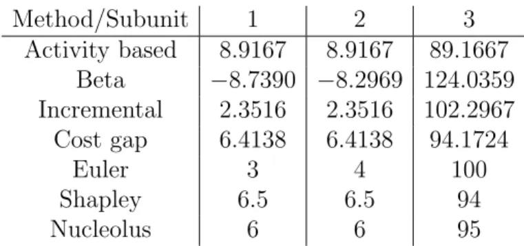
Example 3.1 (Example 2.1 continued.). Table 2 shows the allocated risk cap- ital by the above given seven methods for the risk capital allocation situation of Example 2.1.
Method/Subunit 1 2 3
Activity based 8.9167 8.9167 89.1667 Beta −8.7390 −8.2969 124.0359 Incremental 2.3516 2.3516 102.2967 Cost gap 6.4138 6.4138 94.1724
Euler 3 4 100
Shapley 6.5 6.5 94
Nucleolus 6 6 95
Table 2: The allocated risk capital of Example 2.1.
In this example, in case of the Beta method the betas are −0.0817,
−0.0775 and 1.1592 respectively, while in case of the Cost gap method the gammas are 8, 8 and 13 respectively.
4 Properties of the allocation methods
In this section we present our analytical and simulations results. It is im- portant that we use a general coherent measure of risk, that is we test the fairness requirements for any coherent measure of risk.
4.1 Analytic results
Table 3 summarizes our analytical results. The interpretation of the table is as follows: the √
sign means that the method in the given row meets the fairness property of the column. Before we detail our results, we note that the result of Cs´oka and Pint´er (2011) (see Theorem 2.3) implies that none of the methods meets all the three fairness requirements.
Method / Property Core Compatibility Equal Treatment Property Strong Monotonicity
Activity based ∅ √
∅
Beta ∅ ∅ ∅
Incremental ∅ √
∅
Cost gap ∅ √
∅
Euler ∅ ∅ ∅
Shapley ∅ √ √
Nucleolus √ √
∅
Table 3: Properties of the methods
Let us move to the detailed results. The definition of the Activity based method implies that it satisfies Equal Treatment Property, and as our sim- ulations results show (Section 4.2) it does not satisfy Core Compatibility.
Regarding Strong Monotonicity we provide the following example.
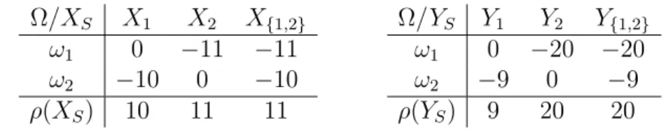
Example 4.1. Let us consider risk capital allocation situations XNρ and YNρ, where for both cases we have Ω = {ω1, ω2}, Mdenotes all subsets of Ω, and P is such that P({ω1}) = P({ω2}) = 12. Moreover, we have two subunits, N ={1,2}, and the applied measure of risk,ρis the 50%-Expected Shortfall (the maximum loss again). The vectors Xi and Yi and their sums are in Table 4.
Ω/XS X1 X2 X{1,2}
ω1 0 −11 −11 ω2 −10 0 −10 ρ(XS) 10 11 11
Ω/YS Y1 Y2 Y{1,2}
ω1 0 −20 −20 ω2 −9 0 −9 ρ(YS) 9 20 20
Table 4: The Activity based and the Beta methods do not satisfy Strong Monotonicity.
Here ρ(X1) = 10 ≥ 9 = ρ(Y1) and ρ(XN)−ρ(X2) = 0 ≥ 0 = ρ(YN)− ρ(Y2), but ϕAB1 (XNρ) = 102111 < 299 20 = ϕAB1 (YNρ), so the Activity based method does not satisfy Strong Monotonicity.
The Beta method does not meet any of the considered fairness require- ments. Example 3.1 shows that it does not satisfy Equal Treatment Property, as it allocates different amounts of capital to subunits 1 and 2. The simu- lation results also show that it is does not satisfy Core Compatibility, while regarding Strong Monotonicity we provide the following example:
Example 4.2. Consider the situation of Example 4.1. Thenρ(X1) = 10≥9 = ρ(Y1) and ρ(XN)−ρ(X2) = 0≥0 =ρ(YN)−ρ(Y2), but ϕB1(XNρ) =−110<
−16.36 =ϕB1(YNρ), so the Beta method does not meet Strong Monotonicity.
In case of the Incremental method it can also be seen from the defining formula that it satisfies Equal Treatment Property and the simulation results also show that it does not satisfy Core Compatibility. We examine Strong Monotonicity in the following example.
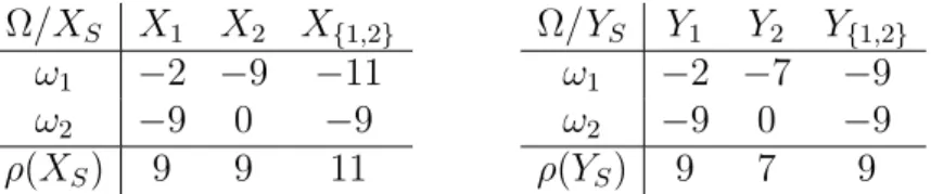
Example 4.3. Let us consider risk capital allocation situations XNρ and YNρ, where for both cases we have Ω = {ω1, ω2}, Mdenotes all subsets of Ω, and P is such that P({ω1}) = P({ω2}) = 12. Moreover, we have two subunits, N ={1,2}, and the applied measure of risk,ρis the 50%-Expected Shortfall (the maximum loss again). The vectorsXi andYi and their sum are in Table 5.
Ω/XS X1 X2 X{1,2}
ω1 −2 −9 −11 ω2 −9 0 −9 ρ(XS) 9 9 11
Ω/YS Y1 Y2 Y{1,2}
ω1 −2 −7 −9 ω2 −9 0 −9 ρ(YS) 9 7 9
Table 5: The Incremental method does not satisfy Strong Monotonicity.
Here ρ(X1) = 9 = ρ(Y1) and ρ(XN)−ρ(X2) = 2 = ρ(YN)−ρ(Y2), but ϕN1 (XNρ) = 112 < 9 = ϕN1 (YNρ), so the Incremental method does not satisfy Strong Monotonicity.
The Cost gap method is very similar to the Incremental method, by definition it also meets Equal Treatment Property and the simulation results also show that it does not satisfy Core Compatibility. Regarding Strong Monotonicity we provide the following example:
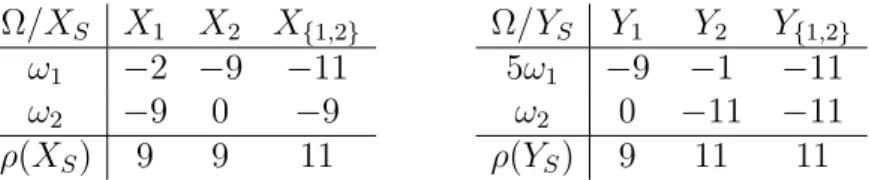
Example 4.4. Let us consider risk capital allocation situations XNρ and YNρ, where for both cases in the probability field (Ω,M, P) we have that Ω = {ω1, ω2},Mdenotes all subsets of Ω, andP is such thatP({ω1}) = P({ω2})
= 12, we have two subunits, N ={1,2}, and the applied measure of risk,ρis the 50%-Expected Shortfall (the maximum loss again). The vectors Xi and Yi and their sum are shown in Table 6.
Here ρ(X1) = ρ(Y1) and ρ(XN) − ρ(X2) = 2 = ρ(YN)− ρ(Y2), but ϕCG1 (XNρ) = 112 > 92 = ϕCG1 (YNρ), so the Cost gap method does not fulfill Strong Monotonicity.
In case of the Euler method Buch and Dorfleitner (2008) proved that for differentiable coherent measures of risk the Euler method satisfies Core
Ω/XS X1 X2 X{1,2}
ω1 −2 −9 −11 ω2 −9 0 −9 ρ(XS) 9 9 11
Ω/YS Y1 Y2 Y{1,2}
5ω1 −9 −1 −11 ω2 0 −11 −11 ρ(YS) 9 11 11
Table 6: The Cost gap method does not satisfy Strong Monotonicity.
Compatibility. However, Example 2.1 shows that it does not meet Equal Treatment Property, and generally the method does not satisfy any of the fairness requirements.
Example 4.5. Consider the situations of Example 4.3, thenρ(X1) = 9 =ρ(Y1) and ρ(XN)−ρ(X2) = 2 =ρ(YN)−ρ(Y2), but ϕE1(XNρ) = 2 < 9 = ϕE1(YNρ).
Moreover, ϕE2(YNρ) = 7, that is ϕE1(YNρ) +ϕE2(YNρ) = 16 > 9 = ρ(YN), so the Euler method satisfies neither Equal Treatment Property, nor Strong Monotonicity, nor Core Compatibility. Core Compatibility fails since in this example the measure of risk is not differentiable.
The properties of the Shapley method are described in Cs´oka and Pint´er (2011), they show that it is the only efficient method (allocating all the risk of the main unit) while meeting both Equal Treatment Property and Strong Monotonicity, but not Core Compatibility. It is also well-known that the Nucleolus method meets Equal Treatment Property and Core Compatibility, but Young (1985) shows a counterexample (p. 69), where it does not meet Strong Monotonicity2.
Summarizing our results we can say that the best performing methods are the game theoretic methods: the Shapley method and the Nucleolus method, as both of them satisfy exactly two of the three fairness requirements.
4.2 Simulation results
How often is in practice one of the properties of Core Compatibility, Equal Treatment Property and Strong Monotonicity violated? As the Shapley method is the only efficient method meeting both Equal Treatment Prop- erty and Strong Monotonicity (Cs´oka and Pint´er, 2011), checking its average Core Compatibility for return distributions having empirically observable characteristics can give an answer.
In the simulations we model the returns of a financial unit (for instance a bank) consisting of, at first, three, then four subunits (for instance divisions),
2Actually, Young (1985)’s counterexample says more, it shows that Core Compati- bility and Strong Monotonicity contradict each other (for more about this contradiction regarding risk allocation games see Cs´oka and Pint´er (2011))
assuming each has invested into assets worth $100 million. We generate re- turn time series using random correlation matrices. As a first approach, we use normal distribution, but we also run the simulations with Student’s t- distribution (hencefortht-distribution). From the simulated returns changes in the invested values, from them risks of the coalitions (1 %-Expected Short- fall) can be calculated.
It is necessary to include the t-distribution, since in practice extremely low and high returns occur more often than it is implied by the normal distribution. That is, the tails of the distribution are heavier than of the normal distribution (Cont, 2001). This is called the stylized fact of heavy tails, first observed by Mandelbrot (1963) on cotton prices. The parameter of the t-distribution, the degrees of freedom (from now on ν) shows how heavy the tails are. The lower the degrees of freedom the heavier the tails are. We run the simulations using t-distributions with ν = 3 (following the “cubic law of returns”) and with ν = 10 (lighter tail). To analyze at the effects of the fat tail we check average Core Compatibility of all the seven methods, except the Nucleolus method and the Euler method defined by Boonen et al.
(2012), since we know that they satisfy Core Compatibility all the time.
In order to get the return series we first generate correlation matrices (more precisely, first Cholesky matrices) and the standard deviations of the assets. For each correlation matrix we generate a lower triangular matrix consisting of elements uniformly distributed on the interval (−1,1). We multiply this by its transpose and we normalize the matrix – this way we get the correlation matrix. The standard deviations are generated from the interval (0.01,0.04) by using uniform distribution.
Then, we generate at first three, then four independent normally and t- distributed time series (with a mean of zero and a variance of one) consisting of 1000 elements, that we multiply by the Cholesky matrices and the standard deviations. This way finally we get multivariate normal and t-distributions.
We generate Cholesky matrices 100000 times and for all Cholesky matrices a random return series consisting of 1000 elements. In the determination of the iteration number we consider both the running time (3-6 minutes for each setting) and the stability of the0 results (the precision is around 0.3 %).
We choose to generate return series consisting of 1000 elements, because it equals four years of return data (assuming to have 250 trading days a year) considered to be enough for more or less exact risk assessment.
Our aim, similarly to Homburg and Scherpereel (2008) is to determine the proportion of the examined cases resulting allocations in the core. Nev- ertheless, contrary to them, we choose a coherent measure of risk, Expected Shortfall, not Value at Risk and we do not consider only the normal distri- bution. Furthermore, we examine more risk capital allocation methods than
they do. Naturally, the closer is the ratio of Core Compatibility to 100% the better the method is.
Table 7 shows the rounded results for three players.
Method/Distribution Normal t-distr. (ν= 10) t-distr. (ν = 3)
Activity based 26.2% 26.5% 27.6%
Beta 80.8% 74.3% 57.8%
Incremental 20.3% 19.5% 19.4%
Cost gap 99.8% 99.7% 99.1%
Euler 100% 100% 100%
Shapley 59.3% 57.1% 57.1%
Nucleolus 100% 100% 100%
Table 7: Average Core Compatibility in case of three subunits
As Table 7 shows the Cost gap, the Euler and the Nucleolus methods perform much better than the other four methods. The Incremental and the Activity based methods show relatively poor performance, but the Shapley and the Beta methods also obey the criterion of Core Compatibility in a large proportion of the cases.
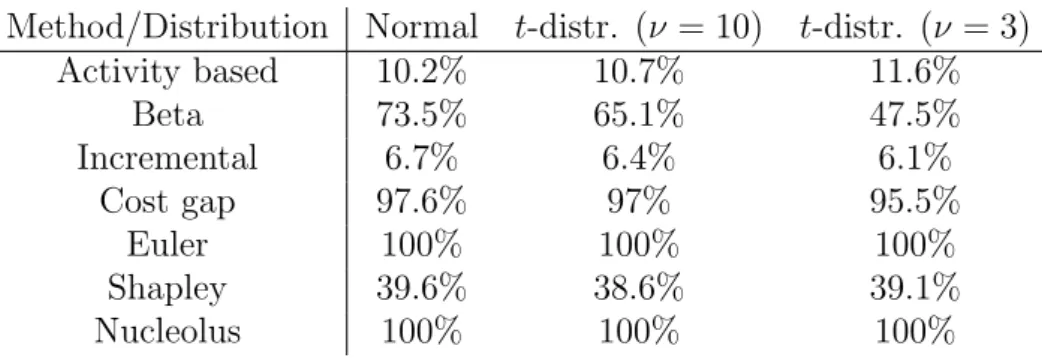
Table 8 shows our simulation results for four players.
Method/Distribution Normal t-distr. (ν= 10) t-distr. (ν = 3)
Activity based 10.2% 10.7% 11.6%
Beta 73.5% 65.1% 47.5%
Incremental 6.7% 6.4% 6.1%
Cost gap 97.6% 97% 95.5%
Euler 100% 100% 100%
Shapley 39.6% 38.6% 39.1%
Nucleolus 100% 100% 100%
Table 8: Average Core Compatibility in case of four subunits
Comparing the ratios of core allocations with four players to our previ- ous results with three players we can generally say that the ratio of core allocations is weakly decreasing as we increase the number of players. The intuition might be that with more players the core itself gets smaller.
Let us consider the tendencies with respect to the fatness of the tails.
Starting at the normal distribution and decreasing the degrees of freedom of the t-distribution we get fatter tails. The fatter the tails the lower the Core Compatibility of the methods tends to be, except for the activity based method and the Shapley method in case of four subunits. Thus the more
extreme events usually generate more extreme claims of the coalitions, which are usually harder to satisfy.
Using the 5%-Expected Shortfall there is at most 2 % change in Core Compatibility, except for the Beta method where we can have 10-20 % higher numbers.
The results of the simulations with four players outline the fact that if we look for a suitable method for practical applications regarding Core Compatibility, the only possible candidates are the Cost gap, the Euler and the Nucleolus methods. The low ratio of the Shapley method shows that the impossibility of fair risk allocation is indeed a practical problem (compare it to Theorem 2.3).
Our general conclusion is the following. Even if we are not mainly in- terested in Core Compatibility, we have only a few relevant alternatives left.
Our analytic results in Table 3 show that only two methods satisfy more than one of the three axioms: the Shapley and the Nucleolus methods. As the Shapley method is the only efficient method meeting both Equal Treatment Property and Strong Monotonicity (Cs´oka and Pint´er, 2011), the low ratio of the Shapley method’s Core Compatibility means that in practical appli- cations we really have to give up one of the three fairness requirements, so there is no ideal risk allocation method in practice either.
References
Acerbi C, Scandolo G (2008) Liquidity risk theory and coherent measures of risk. Quantitative Finance 8:681–692
Acerbi C, Tasche D (2002) On the Coherence of Expected Shortfall. Journal of Banking and Finance 26:1487–1504
Artzner PF, Delbaen F, Eber JM, Heath D (1999) Coherent Measures of Risk. Mathematical Finance 9:203–228
Aumann RJ, Shapley LS (1974) Values of non-atomic games. Princeton Uni- versity Press
Boonen T, De Waegenaere A, Norde H (2012) A generalization of the Aumann-Shapley value for risk capital allocation problems. CentER Dis- cussion Paper Series No. 2012-091
Buch A, Dorfleitner G (2008) Coherent risk measures, coherent capital allo- cation and the gradient allocation principle. Insurance: Mathematics and Economics 42(1):235–242
Cont R (2001) Empirical properties of asset returns: Stylized facts and sta- tistical issues. Quantitative Finance 1:223–236
Cs´oka P, Pint´er M (2011) On the impossibility of fair risk allocation. IEHAS Discussion Papers 1117, Institute of Economics, Centre for Economic and Regional Studies, Hungarian Academy of Sciences.
Cs´oka P, Herings PJJ, K´oczy L ´A (2007) Coherent Measures of Risk from a General Equilibrium Perspective. Journal of Banking and Finance 31(8):2517–2534
Cs´oka P, Herings PJJ, K´oczy L ´A (2009) Stable Allocations of Risk. Games and Economic Behavior 67(1):266–276
Denault M (2001) Coherent Allocation of Risk Capital. Journal of Risk 4(1):1–34
Driessen TSH, Tijs SH (1986) Game theory and cost allocation problems.
Management Science 32 (8), 1015–1028.
Hamlen SS, Hamlen WA, Tschirthart JT (1977) The Use of Core Theory in Evaluating Joint Cost Allocation Schemes. The Accounting Review 52:616–627
Homburg C, Scherpereel P (2008) How Should the Joint Capital be Allocated for Performance Measurement? European Journal of Operational Research 187(1):208–227
Jorion P (2007) Value at Risk: The New Benchmark for Managing Financial Risk. McGraw - Hill
Kalkbrener M (2005) An Axiomatic Approach to Capital Allocation. Math- ematical Finance 15(3):425–437
Kim JHT, Hardy MR (2009) A capital allocation based on a solvency ex- change option. Insurance: Mathematics and Economics 44(3):357–366 Krokhmala P, Zabarankin M, Uryasev S (2011) Modeling and optimization
of risk. Modeling and optimization of risk Surveys in Operations Research and Management Science 16(2):49–66
Mandelbrot B (1963) The Variation of Certain Speculative Prices. The Jour- nal of Business 36(4):394–419
Schmeidler D (1969) The Nucleolus of a Characteristic Function Game. SIAM Journal on Applied Mathematics 17:1163–1170
Shapley LS (1953) A value for n-person games. In: Kuhn HW, Tucker AW (eds) Contributions to the Theory of Games II, Annals of Mathematics Studies, vol 28, Princeton University Press, Princeton, p 307–317
Valdez E, Chernih A (2003) Wang’s capital allocation formula for ellipti- cally contoured % distributions. Insurance: Mathematics and Economics 33:517–532
Young HP (1985) Monotonic Solutions of Cooperative Games. International Journal of Game Theory 14:65–72