On the impossibility of fair risk allocation ∗
P´ eter Cs´ oka
†, Mikl´ os Pint´ er
‡Corvinus University of Budapest
November 7, 2010
Abstract
Measuring and allocating risk properly are crucial for performance evaluation and internal capital allocation of portfolios held by banks, insurance companies, investment funds and other entities subject to financial risk. We show that by using a coherent measure of risk it is impossible to allocate risk satisfying the natural requirements of (Solution) Core Compatibility, Equal Treatment Property and Strong Monotonicity. To obtain the result we characterize the Shapley value on the class of totally balanced games and also on the class of exact games.
Keywords: Coherent Measures of Risk, Risk Allocation Games, To- tally Balanced Games, Exact Games, Shapley value, Solution core JEL Classification: C71, G10
1 Introduction
If a financial enterprise (bank, insurance company, investment fund, etc.) consists of divisions (individuals, products, subportfolios, etc.), not only is it
∗P´eter Cs´oka thanks thanks funding by the project T ´AMOP/4.2.1/B-09/1/KMR-2010- 0005. Mikl´os Pint´er thanks the Hungarian Scientific Research Fund (OTKA) and the J´anos Bolyai Research Scholarship of the Hungarian Academy of Sciences for the financial support.
†Department of Finance, Corvinus University of Budapest, 1093 Hungary, Budapest, F˝ov´am t´er 8., peter.csoka@uni-corvinus.hu
‡Department of Mathematics, Corvinus University of Budapest, 1093 Hungary, Bu- dapest, F˝ov´am t´er 13-15., miklos.pinter@uni-corvinus.hu
important tomeasureproperly the risk of the main entity, but also toallocate the diversification benefits to the divisions. Risk allocation can be used for at least two purposes: for performance evaluation or for allocating internal capital requirements. In the first case risk is used to calculate risk adjusted returns for performance evaluation, which crucially depends on the allocated risk. In the second case the measure of risk is used to determine capital requirements, which serve as a cushion against default. Holding capital is costly, hence capital allocation is also important in this case.
To measure risk appropriately we applycoherent measures of risk (Artzner et al., 1999) defined by four axioms: monotonicity, subadditivity, positive homogeneity, and translation invariance. These axioms are supported by a natural general equilibrium approach to measure risk (Cs´oka et al., 2007).
Moreover, Acerbi and Scandolo (2008) justify the axioms to incorporate liq- uidity risk as well. Of these axioms, subadditivity captures the notion that the risk of the main unit is at most as large as the sum of the risks of the divisions, since there is a diversification effect.
Risk allocation games (Denault, 2001) are transferable utility cooperative games defined to model the allocation of diversification benefits. When using a coherent measure of risk, Cs´oka et al. (2009) show that every risk allocation game is atotally balanced game, and that there exits a coherent risk measure such that the class of risk allocation games defined by this coherent risk measure coincides with the class of totally balanced games. In other words, the four axioms of coherent measure of risk allows a risk measure such that the class of risk allocation games defined by this risk measure coincides with the class of totally balanced games. Cs´oka et al. (2009) also prove that the class of risk allocation games with no aggregate uncertainty equals the class of exact games in the above sense.
A totally balanced game is a cooperative game having a non-empty core in all of its subgames. Some other applications of totally balanced games are as follows: market games (Shapley and Shubik, 1969), linear production games (Owen, 1975), a class of maximum flow problems (Kalai and Zemel, 1982a), generalized network problems (Kalai and Zemel, 1982b), controlled mathematical programming problems (Dubey and Shapley, 1984), permuta- tion games of less than four players (Tijs et al., 1984), and a special case of market games with a continuum of indivisible commodities: cooperation in fair division (Legut, 1990).
On top of coinciding with risk allocation games with no aggregate uncer- tainty,exact games are studied with a coalitional structure in Casas-M´endez et al. (2003), they arise from multi-issue allocation games (Calleja et al., 2005) and multi-choice games (Branzei et al., 2009).
The risk allocation problem in the framework of cooperative game theory
is the problem of choosing a solution for the given games. In this paper we use perhaps the most popular one-point solution concept of cooperative games: the Shapley value (Shapley, 1953).
In a risk allocation game, anallocation rule shows how to share the diver- sification benefits of the main unit among the divisions, which has of course consequences on the performance evaluation or on the amount of capital allocated. In this paper besides having a none-empty core, (1) Core Com- patibility, we consider three other reasonable properties which a “fair” risk allocation rule should meet. Young (1985) has characterized the Shapley value on the class of all games as the only method satisfying (2) Pareto Op- timality (also called Efficiency), (3) Equal Treatment Property (also called Symmetry) and (4) Strong Monotonicity. In our opinion, these axioms are very natural requirements for a “fair” allocation rule. We interpret them as follows.
Core Compatibility is satisfied if all the risk of the main unit is allocated in such a way that no coalitions of the divisions would like to object their allocated risk capital, by saying that their risk is less than the sum of the risks allocated to the members of the particular coalition.
Pareto Optimality is implied by Core Compatibility, since it requires that all the risk of the main unit should be allocated.
Equal Treatment Property makes sure that similar divisions are treated symmetrically, that is if two divisions make the same marginal risk contribu- tion to all the coalition of divisions not containing them, then the rule should allocate them the very same risk capital.
Strong Monotonicity requires that if the risk environment changes in such a way that the marginal contribution of a division is not decreasing, then its allocated risk capital should not decrease either.
Equal Treatment Property and Strong Monotonicity both capture the idea that the risk of a portfolio depends on the other assets present in the economy, a notion that is formulated in the Capital Asset Pricing Model (Sharpe, 1964; Lintner, 1965).
We show that the last three axioms characterize the Shapley value on the class of totally balanced games and also on the class of exact games. Since the Shapley value is known to be not core compatible on those classes of games, we conclude that there is no risk allocation rule which meets the axioms of Core Compatibility, Equal Treatment Property and Strong Monotonicity.
The challenge in the proof is that the original axiomatization by Young (1985) was proved on the class of all games. Here we have two subclasses (totally balanced games and exact games), it is not even guaranteed that the same axiomatization holds true. We demonstrate that the original proof can not be adopted, we only succeed by using the result of Pint´er (2009).
The other axiomatic approaches in the literature are related to our work are as follows.
Denault (2001) considers the original axiomatization of the Shapley value by Shapley (1953), and concludes that there is no allocation which satisfies Core Compatibility, Equal Treatment Property, Dummy Player Property (a riskless division should be allocated its stand-alone risk) and Additivity Over Games. However, he does not prove that the original axiomatization is true on the class of totally balanced games, and on top of that Additivity is known to be not a natural requirement.
Valdez and Chernih (2003) show that for elliptically contoured distribu- tions the covariance (or beta) method satisfies Core Compatibility, Equal Treatment Property and Consistency (requiring that that allocation method should be independent of the hierarchical structure of the main unit). How- ever, Kim and Hardy (2009) show that it is not even true that the covariance method satisfies Core Compatibility in their setting. Moreover, profit and loss distributions of financial assets are not elliptically contoured, but heavy tailed (Cont, 2001), hence our approach is more general by not restricting the probability distributions.
Kalkbrener (2005) shows that Linear Aggregation, Diversification and Continuity characterizes the gradient principle (or Euler method, where risk is allocated as a result of slightly increasing the weight of all the divisions) to be the only allocation which satisfies those requirements. Although those requirements are also natural, they are not related to the marginalistic re- quirements of Equal Treatment Property and Strong Monotonicity. In fact Kalkbrener (2005) explicitly assumes that the risk allocated to a division does not depend on the decomposition of the other divisions, only on the main unit. There is a related impossibility result by Buch and Dorfleitner (2008). They show that if one uses the gradient principle to allocate risk and Equal Treatment Property is satisfied, then the measure of risk must be linear, not allowing for any diversification benefits.
Our result is tight in the sense that we consider a reasonable weaken- ing of the above listed four axioms of risk allocation. We try to save the requirements of Core Compatibility, Equal Treatment Property and Strong Monotonicity by weakening the Core Compatibility requirement as follows.
If a coalition of divisions blocks an allocation, then in the resulting sub- game the original allocation rule (solution) is applied, and each division should get more in the subgame than in the blocked allocation. This way the divisions think one step ahead, and only object an allocation if all of them individually will get more than before, after applying the same solution for allocating risk. It is straightforward that it is easier for an allocation to be
in the resulting core concept, which we call the solution core.
If we would like to satisfy Pareto Optimality (also implied by Solution Core Compatibility) Equal Treatment Property and Strong Monotonicity, we would have to allocate risk using the Shapley value, and it should be in the Shapley core. However, we show an example for a risk allocation game in which the Shapley value is not in the Shapley core either, thus we can conclude it is also impossible to allocate risk using Solution Core Compatibility, Equal Treatment Property and Strong Monotonicity.
The setup of the paper is as follows: in the following section we introduce the concept of risk allocations games. In Section 3 we present our impos- sibility result, and the last section concludes briefly. The technical part of Section 3 is relegated to the Appendix.
2 Risk allocation games
To define risk allocation games we use the setup of Cs´oka et al. (2009). Let S denote the finite number of states of nature and consider the set RS of realization vectors. State of nature s occurs with probability ps >0, where PS
s=1ps = 1. The vector X ∈ RS represents a division’s possible profit and loss realizations at a given time in the future. The amountXsis the division’s payoff in state of nature s. Negative values of Xs correspond to losses.
A measure of risk is a function ρ : RS → R measuring the risk of a division from the perspective of the present.
Definition 2.1. A function ρ:RS →Ris called a coherent measure of risk (Artzner et al., 1999) if it satisfies the following axioms:
1. Monotonicity: for all X, Y ∈ RS such that Y ≥ X, we have ρ(Y) ≤ ρ(X).
2. Subadditivity: for allX, Y ∈RS, we have ρ(X+Y)≤ρ(X) +ρ(Y).
3. Positive homogeneity: for all X ∈ RS and h ∈ R+, we have ρ(hX) = hρ(X).
4. Translation invariance: for all X ∈ RS and a ∈ R, we have ρ(X + a1S) = ρ(X)−a.
For the interpretation of the axioms see Acerbi and Scandolo (2008), who justify them to incorporate liquidity risk as well.
A well known coherent measure of risk is the maximum loss (Acerbi and Tasche, 2002).
Definition 2.2. Let the outcomes be equiprobable. The maximum loss of the realization vector X is defined by
ML(X) =−min
s∈S Xs. (1)
Suppose a financial enterprise hasn divisions. We study if the risk of the main unit as measured by a coherent measure of risk can be allocated to its constituents satisfying certain requirements to be defined in Definition 3.2.
The required cooperative game theoretical definitions are as follows.
LetN ={1, . . . , n}denote a finiteset of players. A cooperative game with transferable utility (game, for short) is given by avalue function v : 2N →R with v({∅}) = 0. The class of games with player set N is denoted byGN.
An allocation is a vector x ∈Rn, where xi is the payoff of player i ∈N. An allocation x yields payoff x(C) = P
i∈Cxi to a coalition C ∈ 2N. An allocation x ∈ Rn is called Pareto Optimal1, if x(N) = v(N); Individually Rational, if xi ≥ v({i}) for all i ∈ N, and Coalitionally Rational if x(C) ≥ v(C) for all C ∈ 2N. The core (Gillies, 1959) is the set of Pareto Optimal and Coalitionally Rational allocations. The core of game v is denoted by core (v).
For a gamev ∈ GN and a coalitionC ∈2N,asubgame (C, vC) is obtained by restricting v to subsets of C.
Definition 2.3. A game is totally balanced, if its each subgame has a non- empty core.
Let GtbN denote the class of totally balanced games with player set N. An interesting subclass of totally balanced games is the class of exact games (Shapley, 1971; Schmeidler, 1972).
Definition 2.4. A game v ∈ GN is exact, if for each C ∈ 2N there exists a core allocation x such thatx(C) =v(C).
LetGeN denote the class of exact games with player setN.
Resuming to risk allocation, let the matrix of realization vectors corre- sponding to the divisions be given by X ∈RS×n, and let X·i denote the i-th column of X, the realization vector of division i. For a coalition of divisions C ∈2N, letXC = P
i∈C
X·i.
Definition 2.5. Arisk environment is a tuple (N, S, p, X, ρ), whereN is the set of divisions, S indicates the number of states of nature, p= (p1, . . . , pS) is the vector of realization probabilities of the various states, X is the matrix of realization vectors, and ρ is a coherent measure of risk.
1In this paper we use the term Pareto Optimal instead of Efficient.
A risk allocation game assigns to each coalition of divisions the risk in- volved in the aggregate portfolio of the coalition.
Definition 2.6. Given a risk environment (N, S, p, X, ρ) a risk allocation game is a game v ∈ GN, where the value function v : 2N →Ris defined by
v(C) =−ρ(X(C)) for all C ∈2N. (2) A risk allocation game withnplayers is induced by the number of states of nature, their probability of occurrence, n realization vectors and a coherent measure of risk. Let GrN denote the family of risk allocation games with player set N. In such a game, according to Equation (2), the larger the risk of any subset of divisions, the lower its value. We illustrate the definition of the risk allocation game by the following example.
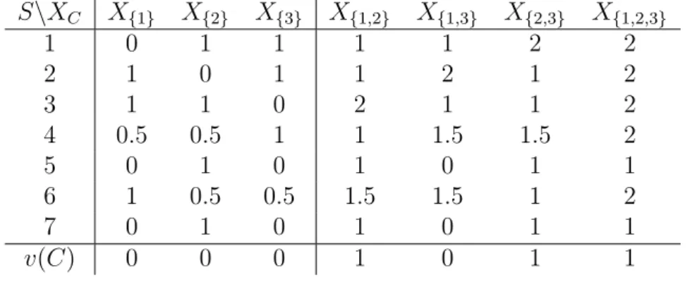
Example 2.7. Consider the following risk environment (N, S, p, X, ρ). We have 3 divisions, 7 states of nature with equal probability of occurrence.
Risk is calculated using the matrix of realization vectors (see Table 1) and the maximum loss (Definition 2.2).
S\XC X{1} X{2} X{3} X{1,2} X{1,3} X{2,3} X{1,2,3}
1 0 1 1 1 1 2 2
2 1 0 1 1 2 1 2
3 1 1 0 2 1 1 2
4 0.5 0.5 1 1 1.5 1.5 2
5 0 1 0 1 0 1 1
6 1 0.5 0.5 1.5 1.5 1 2
7 0 1 0 1 0 1 1
v(C) 0 0 0 1 0 1 1
Table 1: The matrix of realization vectors of a risk environment and the resulting totally balanced risk allocation game v using the maximum loss.
Note that for all C ∈ 2N \ {∅} the value function is given by v(C) =
−ρ(X(C)) = min
s∈S Xs.
If the rows of a matrix of realization vectors sum up to the same number, then there is no aggregate uncertainty. Formally:
Definition 2.8. A matrix of realization vectors X ∈RS×n has no aggregate uncertainty, if there exists a numberα ∈Rsuch that X(N) =α1S.
If there is no aggregate uncertainty, let GrnauN denote the family of risk allocation games with player set N.
Theorem 2.9. (Cs´oka et al., 2009) The class of risk allocation games coin- cides with the class of totally balanced games, that is GrN = GtbN. Moreover, the class of risk allocation games with no aggregate uncertainty equals the class of exact games, that is GrnauN =GeN.
Note that by Theorem 2.9 all risk allocation games are totally balanced (also the one in Example 2.7), and if there is no aggregate uncertainty all of them are exact. Moreover, there exists a coherent risk measure such that for any totally balanced (exact game) there is a risk environment (with no ag- gregate uncertainty) – with the given coherent risk measure – that generates the given game.
This remark can be used to simulate a random totally balanced or exact game by randomizing the risk environment. Using the simulation one can verify if a certain property is satisfied by a random totally balanced or exact game; or if it is not satisfied, one can easily get a counterexample (Example 3.9) or a feeling about the percentage at which a certain requirement is violated.
Next, we study what kind of requirements should be satisfied when allo- cating the diversification benefits (due to the subadditivity axiom of coherent measures of risk in Definition 2.1) in a risk allocation game.
3 Properties of risk allocation rules
A risk allocation rule shows how to share the risk of the main unit among the divisions. In this section we analyze risk allocation rules.
First, we introduce further notations: |N| is for the cardinality of setN, A ⊂ B means A ⊆ B and A 6= B. Moreover, we use |a| for the absolute value of a∈R.
Letv ∈ GN and i ∈N be a game and a player, and ∀S ⊆N let v0i(S) = v(S ∪ {i})−v(S). Then vi0 : 2N \ {N} → R is called player i’s marginal contribution function in game v. Alternatively, vi0(S) is player i’s marginal contribution to coalition S in game v. Player i is a null-player in game v, if v0i = 0.
Moreover, playeriandj are symmetric in gamev,i∼v j, if∀S ⊆N such that i, j /∈ S: vi0(S) = vj0(S). Furthermore, if S ⊆ N is such that ∀i, j ∈S:
i∼v j, then we say that S is an equivalence set in v.
A game v ∈ GN is strictly convex if ∀i ∈ N, ∀T, Z ⊆ N \ {i} such that Z ⊂T: vi0(Z)< v0i(T).
Throughout the paper we consider single-valued solutions. A function ψ : A →RN, defined on A ⊆ GN, is called a solution on the class of games A. In the context of risk allocation problems, we refer to solutions as risk allocation rules.
For arbitrary game v ∈ GN the Shapley solution φ is given by φi(v) = X
S⊆N\{i}
v0i(S)|S|!(|N\S| −1)!
|N|! i∈N,
where φi(v) is also called the Shapley value (Shapley (1953)) of player i in game v.
We illustrate the marginal contribution function and the fact that the Shapley value is not always in the core by continuing Example 2.7.
Example 3.1. Consider the risk allocation game in Example 2.7.
C ∅ {1} {2} {3} {1,2} {1,3} {2,3} {1,2,3}
v(C) 0 0 0 0 1 0 1 1
v10(C) 0 0 1 0 0 0 0
v20(C) 0 1 0 1 0 1 0
v30(C) 0 0 1 0 0 0 0
Table 2: The value function of a risk allocation game and the marginal contribution functions of players 1, 2 and 3.
Note that player 2 has a higher marginal contribution than the others, which is also expressed by the Shapley value, since it isφ(v) = (1/6,2/3,1/6).
However, coalition{1,2}blocks the Shapley allocation, sincev({1,2}) = 1>
1/6 + 2/3 = 5/6.
Next, we introduce the four basic properties (axioms) we recommend a risk allocation rule (solution) should meet.
Definition 3.2. The solution ψ on classA⊆ GN satisfies
• Core Compatibility (CC), if ∀v ∈A: ψ(v)∈core (v),
• Pareto Optimality (P O), if∀v ∈A: P
i∈N
ψi(v) =v(N),
• Equal Treatment Property (ET P), if ∀v ∈ A, ∀i, j ∈ N: (i ∼v j) ⇒ (ψi(v) = ψj(v)),
• Strong Monotonicity (SM), if ∀v, w ∈ A, ∀i ∈ N: (vi0 ≤ wi0) ⇒ (ψi(v)≤ψi(w)).
The financial interpretation of the axioms when applied to a risk alloca- tion rule is as follows.
Core Compatibility is satisfied if a risk allocation is stable, that is all the risk of the main unit is allocated and no coalitions of the divisions would like to object their allocated risk capital, by saying that their risk is less than the sum of the risks allocated to the members of the particular coalition.
Pareto Optimality2 is implied by Core Compatibility, since requires that all the risk of the main unit should be allocated to the divisions.
Equal Treatment Property3 makes sure that similar divisions are treated symmetrically, that is if two divisions make the same marginal risk contribu- tion to all the coalition of divisions not containing them, then the rule should allocate them the very same risk capital.
Strong Monotonicity requires that if the risk environment changes such that the marginal contribution of a division is not decreasing, then its allo- cated risk capital should not decrease either.
Theorem 3.3. (Young, 1985) Let ψ be a solution on the class of all games.
Then solution ψ satisfies P O, ET P and SM if and only if ψ =φ, that is if and only if it is the Shapley solution.
Note that risk allocation games are a proper subset of all games, since they are always totally balanced. We prove a Theorem 3.3 type result on the class of totally balanced games and also on the class of exact games in Theorem 3.4. Formally:
Theorem 3.4. Let ψ be a solution either on the class of totally balanced games or on the class of exact games. Then solution ψ satisfies P O, ET P and SM if and only if ψ =φ, that is if and only if it is the Shapley solution.
The proof of the above theorem is relegated to the Appendix.
The following example shows that Young (1985)’s proof does not work on risk allocation games.
Example 3.5. Let N ={1,2,3,4} and v =u{1,2}+u{2,3}−u{1,2,3}+ 9uN4
2It is also called Efficiency in the literature
3It is also called Symmetry in the literature.
4WhereuT, the unanimity game on coalitionT, is defined as follows: letT ⊆N,T 6=∅ be an arbitrary set, then ∀S⊆N:
uT(S) =
1, ifS⊇T
0 otherwise .
Thenv is an exact game, hence it is totally balanced as well. Notice that player 2 is the only player in game v such that it is not a null-player in any considered unanimity game.
Young (1985)’s proof goes by induction on the number of unanimity games needed to span games. Therefore, in the case of game v assume that on all totally balanced (exact) games spanned by at most three unanimity games the only solution meeting axiomsP O,ET P andSM is the Shapley solution.
Chose player 1 in game v. Then the only considered unanimity game in which player 1 is a null-player is u{2,3}. By leaving out u{2,3}, however, we get gameu{1,2}−u{1,2,3}+ 9uN, which is not totally balanced, hence it is not exact either.
Similarly, chose player 3 in gamev. Then the only considered unanimity game in which player 3 is a null-player is u{1,2}. However, by leaving out u{1,2} we get gameu{2,3}−u{1,2,3}+ 9uN, which is not totally balanced, hence it is not exact either.
Summing up, we cannot make conclusions about the values of players 1, 2 and 3, therefore, Young (1985)’s proof does not work.
It is worth noticing that if|N| ≤ 2, then Young (1985)’s proof works on the class of totally balanced games5, and if |N| ≤3 then that works on the class of exact games6. Since in general, Young (1985)’s proof does not work on the considered classes of games we have to apply a different result: Pint´er (2009)’s proof.
Since the axioms of Definition 3.2 are natural requirements for a risk allocation rule, one can conclude that the only possible way to allocate risk in a “fair” way (satisfying P O, ET P and SM) is to use the Shapley value.
But as we saw in Example 3.1 the Shapley value is not always in the core (and CC implies P O), hence it is impossibly to allocate risk satisfying CC, ET P and SM.
If there is no aggregate uncertainty, we get a proper subset of totally balanced games, exact games. But Rabie (1981) gives an example of a five player exact game, where the Shapley value is also not in the core.7 By Theorem 2.9 this game can be generated by a risk allocation game with no aggregate uncertainty. Thus we can conclude that in case of no aggregate
5Consider game v=u{1,2}+u{2,3}−u{1,2,3} as a counterexample for the three player case.
6It is a slight calculation to see that for any three player exact gamesv=P
T
αTuT,∀T such that|T| ≥2: αT ≥0, which implies that Young (1985)’s proof works.
7It is not too difficult to show that there is no such an example for four or less player exact games, so Rabie (1981)’s counterexample is tight.
uncertainty it is also impossible to allocate risk in a way such that it satisfies CC, ET P and SM.
Our final try to save “fair” allocation rules is to consider an other core concept. In this case if a coalition of divisions blocks an allocation, then in the resulting subgame the original allocation rule is applied (in our case the Shapley value), and each division should get more in the subgame than in the blocked allocation. This way the divisions think one step ahead, and only object an allocation if all of them individually will get more than before, after applying the same allocation rule. Formally:
Definition 3.6. Letψ be an arbitrary solution on set A. The solution core, ψ-core of gamev ∈A is defined as follows: ψ-core (v) =
(
x∈RN
X
i∈N
xi =v(N) and∀S ⊂N such that vS ∈A:ψ(vS)≯xS )
. It is worth noticing that for any game v core (v)⊆ψ-core (v).
Definition 3.7. The solutionψon classA⊆ GN isSolution Core Compatible (ψ-CC) if ∀v ∈A: ψ(v)∈ψ-core (v).
Since we consider risk allocation rules satisfying Pareto Optimality (im- plied by Core Compatibility), Equal Treatment Property and Strong Mono- tonicity, and those requirements characterize the Shapley value, it follows that the risk should also be distributed in the subgame by the Shapley value.
We call this weakened core concept the Shapley core.
To first consider general, totally balanced risk allocation games, let us check if the Shapley value is in the Shapley core in Example 2.7.
Example 3.8. Consider the risk allocation game in Example 2.7. Then by Theorem 2.9 v is a totally balanced game, as we saw in Example 3.1 the Shapley values is φ(v) = (1/6,2/3,1/6), but φ(v{1,2}) = (1/2,1/2). Thus the blocking coalition {1,2} is not formed, the Shapley value is in the Shapley core, since player 2 would be worse off in the subgame v{1,2}. Looking at the risk environment the intuition is that division 2 is a good hedge against both 1 and 3, but when it is only with one of them, then it does not get enough by the Shapley allocation.
However, if we consider an other totally balanced game, we see that the Shapley value is not in the Shapley core either.
Example 3.9. We present a game that is totally balanced and the Shapley value is not in the Shapley core. Consider the following game with three players. Let
v({1}) = v({2}) = v({3}) = 0, v({1,2}) = 27,
v({1,3}) = 19, v({2,3}) = 14, v({1,2,3}) = 30.
It is easy to check thatv is a totally balanced game,φ(v) = (13,10.5,6.5), v{1,2} is totally balanced andφ(v{1,2}) = (13.5,13.5). Thus it is worth for both player 1 and player 2 to deviate and get the Shapley value in subgame v{1,2}, hence the Shapley value is not in the Shapley core.
For exact games, Rabie (1981)’s counterexample works for the Shapley core as well, thus in that example the Shapley value is not in the Shapley core either. We note that for exact games with at most four players the Shapley value is always in the Shapley core, since it is always in the core.
Corollary 3.10. There is no risk allocation rule meeting conditions CC, ET P and SM, and there is no risk allocation rule ψ such that it meets conditions ψ-CC, ET P and SM.
4 Conclusion
In this paper we have presented impossibility results on risk allocation. Ap- plying game theoretical tools to risk allocation problems, we have considered four very natural axioms: CC (Core Compatibility), ET P (Symmetry) and SM (Strong Monotonicity), and we have showed that there is no risk alloca- tion rule meeting all those three axioms. Later, we have weakened condition CC to Solution Core Compatibility (ψ-CC) and have presented the same impossibility result. Our impossibility results are valid even if we consider risk allocation games with no aggregate uncertainty.
Appendix
To prove Theorem 3.4 we will apply the following Theorem characterizing the Shapley value on a subset of games.
Theorem 4.1. Let set A ⊆ GN be such that ∀v ∈ A, ∀k ∈ N and ∀i ∈ N \ {k}: ∃B ⊆A, ∃w∈A and ∃z(i)∈B such that
1. B is M-closed8, that is ∀g ∈ B, ∀S ⊆ N equivalence set in g and
∀j ∈ N \S: ∃h ∈B such that S∪ {j} is an equivalence set in h and h0j =gj0,
2. w0k=v0k and ∀i∈N \ {k}: z(i)0i =wi0.
Then solution ψ on A is P O, ET P and SM if and only if ψ =φ, that is if and only if ψ is the Shapley solution.
Proof. See Pint´er (2009) Theorem 3.3 pp. 4–5.
In case of risk allocation games, if totally balanced games or exact games were M-closed, then we could apply a simplified version of Theorem 4.1.
However, the following examples show that none of the considered classes of games are M-closed.
Example 4.2. (Total balancedness) Let N ={1,2,3}, and ∀T ⊆N let
v(T) =
0, if |T| ≤1 and T 6={3}
10, if T ={3}
20, if |T|= 2 30, if T =N.
One can check that v is a totally balanced game and S ={1,2} is an equiv- alence set in v. However, the only game wsuch that N is an equivalence set in w and w30 =v03, is as follows,∀T ⊆N:
w(T) =
0, if T =∅
10, if |T|= 1 30, if |T|= 2 40, if T =N having an empty core.
(Exactness) Let N ={1,2,3,4}, and ∀T ⊆N let
v(T) =
0, if |T| ≤1
20, if |T|= 2 and 1 ∈T 10, if |T|= 2 and 1 ∈/T 25, if |T|= 3 and 1 ∈T 200, if T ={2,3,4}
222, if T =N.
8M refers to Marginality of solutionψ, requiring that∀v, w∈A, ∀i∈N: (v0i=wi0)⇒ (ψi(v) =ψi(w)). Note that Marginality is implied by Strong Monotonicity.
One can check that v is an exact game and S = {2,3,4} is an equivalence set in v. However, the only game w such that N is an equivalence set in w and w10 =v10 is as follows: ∀T ⊆N let
w(T) =
0, if |T| ≤1 20, if |T|= 2 35, if |T|= 3 57, if T =N.
Game w(T) is not exact, since there is no core allocation giving 0 to any one player coalition (each of the other players should get 20, which is impossible).
It is a slight calculation to see that if |N| ≤ 2, then the class of totally balanced games is M-closed, and if |N| ≤3, then the class of exact games is also M-closed.
The proof of Theorem 3.4. We will proceed in 6 steps and apply Theorem 4.1 by showing that set B can be the class of strictly convex games for both totally balanced games and exact games.
Step 1: Let v ∈ GN be an arbitrary totally balanced / exact game and let k∈N be an arbitrary player. Then let
M ≥max
S⊆N|vk0(S)|+ 2 and ∀S ⊆N let
w(S) =
0, if S =∅
(M|N|)|S|, if S 6=∅ and k /∈S (M|N|)|(S\{k})|+vk0(S\ {k}) otherwise.
(3) Then it is easy to see thatw0k=v0k.
Step 2: Next we show that for any player i∈N\ {k},∀Z ⊂T ⊆N\ {i}:
wi0(T)−wi0(Z)>0 , (4) that is player i has a strictly convex marginal contribution profile.
Three cases can happen:
k∈Z,k /∈T and k∈T \Z. If k∈Z, then
wk0((T \ {k})∪ {i})−w0k(T \ {k})
−wk0((Z\ {k})∪ {i}) +wk0(Z\ {k})>−4M. (5)
Without loss of generality9 we can assume that |N| ≥2.
w((T \ {k})∪ {i})−w(T \ {k})−w((Z\ {k})∪ {i}) +w(Z\ {k})
>4M. (6) Summing up Inequalities (5) and (6) leads to
wi0(T)−wi0(Z)>0.
The proofs of the other two cases (k /∈T and k ∈T \Z) are similar.
Step 3: Next, we show that w has a non-empty core.
∀i∈N let
xi =
( w0k(N \ {k}), if i=k
w(N\{k})
|N\{k}| otherwise. (7)
Next, we show that x is a core allocation.
It is clear thatw(N) = P
i∈N
xi and P
i∈N\{k}
xi =w(N\{k}). Hence coalition N \ {k} cannot block allocationx.
Notice that ∀T ⊆N such that T 6=N \ {k}, and ∀i∈N \ {k}:
xi ≥w(T). (8)
Next, we show that coalition T cannot block allocation x either. Two cases can happen:
(1) k /∈T: Then (remember M ≥1)
xi = (M|N|)|N\{k}|
|N \ {k}| = M|N|
|N \ {k}|(M|N|)|N\{k}|−1
≥(M|N|)|N\{k}|−1 ≥w(T).
(2) k ∈T: Notice that if |N \ {k}| = 1, then the proof is accomplished.
Otherwise, since M ≥2 and |N \ {k}| ≥2
xi = M|N|
|N \ {k}|(M|N|)|N\{k}|−1 ≥M(M|N|)|N\{k}|−1
≥(M|N|)|T\{k}|+M ≥w(T).
9The case of |N|= 1 is trivial.
Step 4: Next we show that ifv is totally balanced, thenwis exact, hence it is totally balanced as well10.
LetS ⊆N be an arbitrary non-empty coalition.
w is exact: ∀i∈N let
yi =
wk0(N \ {k}), if i=k and k /∈S wk0(S\ {k}), if i=k and k∈S
w(S\{k})
|S\{k}| , if i6=k and i∈S
w(N\{k})−w(S)
|N\(S∪{k})| , if i /∈S∪ {k} and k /∈S
w(N)−w(S)
|N\S| , if i /∈S and k ∈S.
Notice that if S=N, then y=x of Equation (7) and it follows from Step 3 that coalition N \ {k} cannot block allocation y. Moreover, it is clear that
P
i∈N
yi = w(N), P
i∈S
yi = w(S) and ∀i ∈ N \(S∪ {k}): yi ≥ xi, where xi is from (7). The construction of wimplies that ify can be blocked, then it can only be blocked via a coalitionT such that T\(S∪ {k})6=∅. However, from Inequality (8) for any i∈T \(S∪ {k}): yi ≥xi ≥w(T), hence (yi)i∈N is in the core of w.
Step 5: Next we construct the game depending on player i, z(i) by re- peating the construction ofw. That is, leti∈N\ {k}be an arbitrary player.
Moreover, for all S ⊆N let
z(i)(S) =
0, if S =∅
(M|N|)|S|, if S 6=∅ and i /∈S (M|N|)|S\{i}|+wi0(S\ {i}) otherwise
,
where M ≥max
S⊆N|wi0(S)|+ 2.
Then it is easy to see that z(i)0i =w0i and z(i) is a strictly convex game.
The class of strictly convex games is anM-closed class of games (see Lemma 3.9 in Pint´er (2009) p. 6).
Step 6: We can apply Theorem 4.1 such that A is the class of totally balanced / exact games and B is the class of strictly convex games.
10Since every exact game is totally balanced, and in the proof we use only thatwk0(S\ {k}) =vk0(S\ {k})≥vk0(∅) =w0k(∅) (which is true for both types of games), it is enough to consider only a gamev such thatvk0(S\ {k})≥v0k(∅).
References
Acerbi C., Scandolo G., 2008. Liquidity risk theory and coherent measures of risk. Quantitative Finance 8, 681–692.
Acerbi C., Tasche D., 2002. On the coherence of expected shortfall. Journal of Banking and Finance 26, 1487–1504.
Artzner P.F., Delbaen F., Eber J.M., Heath D., 1999. Coherent measures of risk. Mathematical Finance 9, 203–228.
Branzei R., Tijs S., Zarzuelo J., 2009. Convex multi-choice games: Charac- terizations and monotonic allocation schemes. European Journal of Oper- ational Research 198, 571–575.
Buch A., Dorfleitner G., 2008. Coherent risk measures, coherent capital allocations and the gradient allocation principle. Insurance: Mathematics and Economics 42 (1), 235–242.
Calleja P., Borm P., Hendrickx R., 2005. Multi-issue allocation situations.
European Journal of Operational Research 164, 730–747.
Casas-M´endez B., Garc´ıa-Jurado I., van den Nouweland A., V´azquez-Brage M., 2003. An extension of the τ-value to games with coalition structures.
European Journal of Operational Research 148, 494–513.
Cont R., 2001. Empirical properties of asset returns: Stylized facts and statistical issues. Quantitative Finance 1, 223–236.
Cs´oka P., Herings P.J.J., K´oczy L. ´A., 2007. Coherent measures of risk from a general equilibrium perspective. Journal of Banking and Finance 31 (8), 2517–2534.
Cs´oka P., Herings P.J.J., K´oczy L. ´A., 2009. Stable allocations of risk. Games and Economic Behavior 67 (1), 266–276.
Denault M., 2001. Coherent allocation of risk capital. Journal of Risk 4 (1), 1–34.
Dubey P., Shapley L.S., 1984. Totally balanced games arising from controlled programming problems. Mathematical Programming 29, 245–267.
Gillies D.B., 1959. Solutions to general non-zero-sum games, vol. IV ofCon- tributions to the Theory of Games. Princeton University Press.
Kalai E., Zemel E., 1982a. Generalized network problems yielding totally balanced games. Operations Research 30, 998–1008.
Kalai E., Zemel E., 1982b. Totally balanced games and games of flow. Math- ematics of Operations Research 7, 476–478.
Kalkbrener M., 2005. An axiomatic approach to capital allocation. Mathe- matical Finance 15 (3), 425–437.
Kim J.H.T., Hardy M.R., 2009. A capital allocation based on a solvency exchange option. Insurance Mathematics and Economics 44, 357–366.
Legut J., 1990. On totally balanced games arising from cooperation in fair division. Games and Economic Behavior 2, 47–60.
Lintner J., 1965. The valuation of risky assets and the selection of risky investments in stock portfolios and capital budgets. Review of Economics and Statistics 47, 13–37.
Owen G., 1975. On the core of linear production games. Mathematical Programming 9, 358–370.
Pint´er M., 2009. Young’s axiomatization of the Shapley value - a new proof.
arXiv:0805.2797v2 .
Rabie M.A., 1981. A note on the exact games. International Journal of Game Theory 10 (3-4), 131–132.
Schmeidler D., 1972. Cores of exact games. Journal of Mathematical Analysis and Applications 40, 214–225.
Shapley L.S., 1953. A value for n-person games. In: H.W. Kuhn, A.W.
Tucker (Eds.), Contributions to the Theory of Games II, vol. 28 ofAnnals of Mathematics Studies. Princeton University Press, Princeton, pages 307–
317.
Shapley L.S., 1971. Cores of convex games. International Journal of Game Theory 1, 11–26.
Shapley L.S., Shubik M., 1969. On market games. Journal of Economic Theory 1, 9–25.
Sharpe W.F., 1964. Capital asset prices: A theory of market equilibrium under conditions of risk. Journal of Finance 19, 425–442.
Tijs S., Parthasarathy T., Potters J., Prassad V.R., 1984. Permutation games: Another class of totally balanced games. OR Spektrum 6, 119–123.
Valdez E.A., Chernih A., 2003. Wang’s capital allocation formula for ellipti- cally contoured distributions. Insurance: Mathematics and Economics 33, 517–532.
Young H.P., 1985. Monotonic solutions of cooperative games. International Journal of Game Theory 14, 65–72.