Surface magnetic activity of the fast-rotating G5-giant IN Comae, central star of the faint planetary nebula LoTr 5 ?

(1)

February 26, 2019

Surface magnetic activity of the fast-rotating G5-giant IN Comae, central star of the faint planetary nebula LoTr 5 ^?

Zs. K˝ovári¹, K. G. Strassmeier², K. Oláh¹, L. Kriskovics¹, K. Vida¹, T. A. Carroll², T. Granzer², I. Ilyin², J. Jurcsik¹, E. K˝ovári³, and M. Weber²

1 Konkoly Observatory, Research Centre for Astronomy and Earth Sciences, Hungarian Academy of Sciences, Konkoly Thege út 15-17., H-1121, Budapest, Hungary; e-mail:kovari.zsolt@csfk.mta.hu

2 Leibniz-Institute for Astrophysics Potsdam (AIP), An der Sternwarte 16, D-14482 Potsdam, Germany

3 Eötvös University, Department of Astronomy, Pf. 32., H-1518, Budapest, Hungary Received ; accepted

ABSTRACT

Context.On the asymptotic giant branch, low to intermediate mass stars blow away their outer envelopes, forming planetary nebulae.

Dynamic interaction between the planetary nebula and its central progenitor is poorly understood. The interaction is even more complex when the central object is a binary star with a magnetically active component, like it is the case for the target in this paper.

Aims.We aim to quantify the stellar surface activity of the cool binary component of IN Com and aim to explain its origin. In general, we need a better understanding of how central binary stars in planetary nebulae evolve and how this evolution could develop such magnetically active stars like IN Com.

Methods.We present a time-series of 13 consecutive Doppler images covering six months in 2017 and use it to measure the surface differential rotation with a cross-correlation method. Hitherto unpublished high-precision photometric data from between 1989 to 2017 are presented. We apply Fourier-transformation based frequency analysis to both photometry and spectra. Very high resolution (R≈200,000) spectra are used to update IN Com’s astrophysical parameters by means of spectral synthesis.

Results. Our time-series Doppler images show cool and warm spots coexisting with an average surface temperature contrast of

−1000 K and+300 K with respect to the effective temperature. Approximately 8% of the stellar surface is covered with cool spots and≈3% with warm spots. A consistent cool polar spot is seen in all images. The average lifetime of the cool spots is not much more than a few stellar rotations (one month), while the warm spots appear to live longer (3 months) and are mostly confined to high latitudes. We found anti-solar surface differential rotation with a shear coefficient ofα =−0.026±0.005 suggesting an equatorial rotation period of 5.973±0.008 d. We reconfirm the 5.9-day rotation period of the cool star from photometry, radial velocities, and Hαline-profile variations. A long-termV-brightness variation with a likely period of 7.2 yr is also found. It appears in phase with the orbital radial velocity of the binary system in the sense brightest at highest velocity and faintest at lowest velocity, that is, at the two phases of quadrature. We redetermine [Ba/Fe], [Y/Fe] and [Sr/Fe] ratios and confirm the overabundance of these s-process elements in the atmosphere of IN Com.

Key words. stars: activity – stars: imaging – stars: late-type – stars: starspots – stars: individual: IN Com

1. Introduction

Undergoing the asymptotic giant branch (AGB) evolution phase, low to intermediate mass stars blow away their outer envelopes, forming planetary nebulae that will be ionized by the develop- ing white dwarfs in their center. However, interaction between the planetary nebula and its central progenitor is far from understood. The scheme is even more complicated, when the central object is a binary star, which may be the majority (e.g., De Marco et al. 2004; Jones & Boffin 2017). When the binary system is em- bedded in a common envelope, the components evolve together, as initially proposed by Paczy´nski (1976). Inside the envelope the stellar cores spiral together and finally they may merge, forming a fast-rotating giant star, such as FK Comae stars (for a recent overview of binary mergers see the contribution by Ph.

Send offprint requests to: Zs. K˝ovári

? Based on data obtained with the STELLA robotic observatory in Tenerife, an AIP facility jointly operated by AIP and the Instituto de Astrofisica de Canarias, and on data acquired with PEPSI using the Vat- ican Advanced Technology Telescope (VATT) jointly operated by AIP and the Vatican Observatory.

Podsiadlowski in González Martínez-País et al. 2014). However, if the envelope material is ejected before merging, the binary evolution may end up in a system involving a white dwarf and a main sequence companion. In this case some of the ejected neb- ular material is captured by the companion, yielding cataclysmic variability, while the accretion gradually spins up the accreting star. In addition, a powerful magnetic dynamo can also develop, since the common envelope is largely convective and supposed to rotate differentially (Tout & Reg˝os 2003). However, the theory of common envelope evolution is extremely complex, involving different physical processes (e.g., ejection, accretion, spiralling, magnetic braking) on different time-scales (thermal, dynami- cal, hydrodynamical, magneto-hydrodynamical, etc.), therefore a self-consistent, all-comprehensive treatment is still not feasi- ble (cf. Podsiadlowski 2001).

In this paper we revisit one of our former Doppler imaging targets, IN Comae (=HD 112313, Strassmeier et al. 1997b, here- after Paper 1), the central object of the faint planetary nebula LoTr 5 (Longmore & Tritton 1980). The system consists of a white dwarf and a giant G-star, which is evident from the com- Article number, page 1 of 18

arXiv:1902.09460v1 [astro-ph.SR] 25 Feb 2019

(2)

posite IUE spectra (Feibelman & Kaler 1983). Actually, the central object is a long-period (Porb ≈2700 d≈ 7.4 yr) binary system, consisting of a rapidly rotating magnetically active G5 giant (vsini=67 kms⁻¹) and a hot (Teff ≈150 000 K) subdwarf companion (cf. Jones et al. 2017, and their references). It was even suggested that the G5 component had a close companion, forming a hierarchical triple system (Jasniewicz et al. 1987; Malasan et al. 1991). However, this option has recently been disproved by Van Winckel et al. (2014), who suggested that either the white dwarf (or hot subdwarf) formed a close binary together with a yet undiscovered star of some 2–3M, or alternatively the orbital plane was not coplanar with the waist of the bipolar nebula. The cool star was found to be barium-rich (Thévenin & Jasniewicz 1997) as a consequence of contamination by s-process elements from the AGB progenitor envelope (cf. Bisterzo et al. 2011), supporting the presumption of spinning-up of the cool component by accreting the ejected envelope material.

Rotational and orbital period determinations of IN Com in the past yielded misinterpretations and even contradictory results. As fundamental period 5.9-day was reported by Noskova (1989), which was attributed to rotation of the G5 giant (see Pa- per 1). However, Malasan et al. (1991) argued for 1.2-day as the most prominent photometric signal (i.e., the 1− f alias of 5.9 days), and also for 1.75 days, based on radial velocity measurements, as a possible orbital period of the assumed close binary.

Jasniewicz et al. (1994) could not confirm this binary orbit, but they claimed that 1.2-day was indeed correct. After a revision, however, Jasniewicz et al. (1996) found the 5.9-day period as more realistic. Oddly, Kuczawska & Mikolajewski (1993) found an even shorter period of 0.25 days, which, however, has not been confirmed ever since. Over and above, the radial velocity measurements in Paper 1 did not support the close binary hy- pothesis. Only recently, Jones et al. (2017) have updated the first reliable orbital motion detection by Van Winckel et al. (2014) and proposed an orbital period of 2717±63 days (≈7.4 years) for the G5 star.

IN Com has been observed in X-rays byXMM-Newtonwith all three European Photon Imaging Cameras (EPIC) on 6 June 2002, and byChandraon 4 December 2002 (Montez et al. 2010).

Spectral fitting shows that the X-ray emission is characterized by two components at about 0.65 keV (both XMM-Newton and Chandra) and at 2.27 and 3.49 keV (XMM-Newton and Chandra, respectively), while the X-ray luminosity was measured as logL_X ≈ 30 erg s⁻¹. Guerrero (2012) fitted theXMM- NewtonEPIC planetary nebula spectrum with 8×10³⁰erg s⁻¹at 0.61 and 3.1 keV, and constructed a spectral energy distribution model from theXMM-Newtondata, the availableIUEspec- tra, and ground based optical and near-infrared photometry. The non-local thermodynamic equilibrium (non-LTE) model showed good agreement with a contribution from a supposed G5 III companion star. It seems, that the X-ray emission dominantly origi- nates from the corona of the magnetically active late-type component of the binary (see Montez et al. 2010, for details).

Our study may contribute in moving towards a better understanding how central binary stars in planetary nebulae evolve and how this evolution could develop such fast-rotating magnetically active stars like IN Com. The paper is organized as follows. In Sect. 2 we present the photometric and spectroscopic observations. In Sect. 3 we provide updated astrophysical parameters for IN Com and present a time-series Doppler imaging study. With that we analyze the spot evolution and measure the surface differential rotation. In Sect. 4 we study the photometric and spectroscopic variability of the IN Com system, while in Sect. 5 the

Hαbehaviour is examined. The results are summarized and dis- cussed in Sect. 6.

2. Observations 2.1. Photometry

Most of the photometric observations were obtained with the T6 and T7 (‘Wolfgang’ and ‘Amadeus’, respectively) 0.75-m automatic photoelectric telescopes (APTs) located at Fairborn Observatory in southern Arizona (Strassmeier et al. 1997a), operated by AIP (Granzer et al. 2001). Altogether 1364 data points were observed in JohnsonV(T6) and 943 in Strömgreny (T7) colours between February 1996–June 2017 (JD 2,450,117–

2,457,911). Besides, 643 JohnsonVobservations were collected with the 1-m RCC telescope of Konkoly Observatory, Budapest, located at Piszkéstet˝o mountain station, Hungary, between Jan- uary 1989–June 1993 (JD 2,447,530–2,449,141). The old photometric data from the literature completed with the new, yet un- publishedVandyobservations are plotted together in Sect. 4 in the top panel of Fig. 6.

2.2. Spectroscopy

Spectroscopic observations were carried out with the 1.2-m STELLA-II telescope of the STELLA robotic observatory (Strassmeier et al. 2010) located at the Izaña Observatory in Tenerife, Spain. It is equipped with the fibre-fed, fixed- format STELLA Echelle Spectrograph (SES) providing an average spectral resolution ofR = 55 000. Altogether 230 high- resolution echelle spectra were recorded between January 26 and June 23, 2017. The spectra cover the 3900–8800 Å wavelength range without gaps. Further details on the performance of the system and the data-reduction procedure can be found in We- ber et al. (2008, 2012) and Weber & Strassmeier (2011). The average signal-to-noise ratio (S/N) of the spectra is 140:1. Ta- ble A.1 in the Appendix summarizes the division of the spectra into 12 independent subsets (dubbed S01–S12) which are used for Doppler imaging.

In addition, 20 ultra-high resolution (R = 200 000) spectra were collected during March 03–15, 2017 with the 1.8-m Vatican Advanced Technology Telescope (VATT) fiber linked to the Potsdam Echelle Polarimetric and Spectroscopic Instru- ment (PEPSI) at the nearby Large Binocular Telescope (LBT).

PEPSI’s characteristics and performance were described by Strassmeier et al. (2015, 2018). With cross disperser (CD) III in the blue arm and CD V in the red arm the set-up provided a wavelength coverage of 4800–5440 Å and 6280–7410 Å, respectively. The 90-min exposures gave typical S/N of 100:1 for the red and 50:1 for the blue wavelength regions. This data set is used primarily to refine some of the fundamental astrophysical parameters of IN Com (see Sect. 3.1). The log for these observations is given in Table A.2 in the Appendix.

3. Doppler imaging

3.1. Adopted stellar parameters

The effective temperature, the surface gravity, the metallicity, and the microturbulence velocity are re-examined by applying the spectrum-synthesis code SME (Piskunov & Valenti 2017) to the ultra-high resolution PEPSI spectra. Our synthesis is based on MARCS model atmospheres (Gustafsson et al. 2008) and assuming local thermodynamic equlibrium (LTE). Atomic param- Article number, page 2 of 18

(3)

eters are taken from the Vienna Atomic Line Database (VALD, Kupka et al. 1999). For the spectrum synthesis we used the 4800–5441 Å and 6278–7419 Å wavelength ranges. SME is applied for all single PEPSI spectra and the individual results are combined in order to estimate their error bars. This way we get Teff=5400±100 K, logg=2.6±0.1, [Fe/H]=−0.10±0.05 and ξmic=2.0±0.4 km s⁻¹for the effective temperature, surface gravity, metallicity and microturbulence, respectively. We note that our temperature and surface gravity values are in good agreement with the recent result by Aller et al. (2018). The radial- tangential macroturbulence dispersion of≈7 km s⁻¹is estimated according to Gray (1981) and Gray & Toner (1986). SME was used to measure the Ba, Y and Sr abundances (cf. Thévenin &

Jasniewicz 1997) as well. For the abundance fits we kept all of the other redetermined astrophysical parameters fixed. We note that for the Ba line fit we take the average of 40 high quality STELLA spectra since the spectral gap between the blue and red arms of the PEPSI data highly overlaps with the 5519–6694 Å region of the 31 neutral and singly ionized barium lines taken from VALD. The new astrophysical data of IN Com are summarized in Table 1.

Table 1.The astrophysical properties of IN Com

Parameter Value

Spectral type G5 III

Gaia distance [pc] 506±12

Vbr[mag] 8.69±0.03

(B−V)_HIP[mag] 0.835±0.004

Mbol[mag] 0.01±0.08

Luminosity [L] 78±6

logg[cgs] 2.6±0.1

Teff [K] 5400±100

vsini[km s⁻¹] 67.0±1.5 Photometric period [d] 5.934±0.001 Equatorial rotation period [d] 5.973±0.008 Differential rotation coefficient −0.026±0.005

Inclination [^◦] 45±15

Radius [R] 11.1⁺_−2.2^5.0

Mass [M] 1.8±0.4

Microturbulence [km s⁻¹] 2.0±0.4 Macroturbulence [km s⁻¹] 7.0 (adopted) Metallicity [Fe/H] −0.10±0.05 Barium/iron ratio [Ba/Fe] 0.85±0.25 Yttrium/iron ratio [Y/Fe] 0.27±0.12 Strontium/iron ratio [Sr/Fe] &1.0

The projected equatorial velocity of 67±1.5 km s⁻¹(Paper 1, but see also Van Winckel et al. 2014) and a 45±15^◦ inclination (cf. Paper 1) together with the equatorial rotation period of 5.973 d (cf. Sect. 4.2) yields a stellar radius of 11⁺_−2.2^5.0R. To- gether withT_e_ff=5400±100 K this radius is consistent with the G5 III classification in the literature.

The new Gaia DR-2 parallax of 1.977±0.046 mas (Gaia Collaboration et al. 2018) yields a distance of 506±12 pc for IN Com. The brightest ever observed V magnitude of 8^m.69± 0^m.03 (see later Fig. 7), while neglecting any interstellar and circumstellar extinction (cf Ciardullo et al. 1999), results in an ab- solute magnitudeMV=0^m.17±0^m.08. This, together with a bolometric correction for a G5 giant of BC = −0^m.163 taken from Flower (1996) gives a bolometric magnitude of M_bol=0^m.01± 0^m.08, and thus a luminosity ofL=78±6Lin fair agreement with the value just from the Stefan-Boltzmann law, but with a

much smaller error bar. Also, taking above radius and our measured gravity the stellar mass is≈1.8±0.4 M.

3.2. Definition of data subsets

The spectroscopic data used for the Doppler-imaging (DI) process are all from the first half of 2017 and are distributed fairly uniformly over the five-months STELLA run. In spite of the rel- atively short rotation period of 5.9 d, we still got satisfactory phase coverage with between 8 and 13 spectra per image for 12 subsequent intervals of typically one stellar rotation each. An additional subset can be formed from the available PEPSI spectra, with a pretty dense phase coverage. Table 2 summarizes the timely distribution of the 13 data subsets (dubbed S01–S12 and P01 for the PEPSI spectra) while Tables A.1 and A.2 in the Ap- pendix record the observing logs for the STELLA and the PEPSI spectra, respectively.

3.3. Image reconstruction with iMap

Our Doppler-imaging codeiMap(Carroll et al. 2012) performs a temperature inversion for a number of photospheric line profiles simultaneously. For the inversions 20 suitable absorption lines were selected from the 5000–6750 Å wavelength range (for the selection criteria see Künstler et al. 2015). Each spectral line is modeled individually and locally, then being disk-integrated and in the final step all disk-integrated line regions are averaged to obtain a mean theoretical profile. These mean profiles are then compared with each observed mean profile (for more details see Sect. 3 in Carroll et al. 2012). For the preparation of the observed mean profile we proceed with a simple S/N-weighted averaging to increase the overall S/N by a factor of≈4.iMapcalculates the local line profiles by solving the radiative transfer with the help of an artificial neural network (Carroll et al. 2008). Atomic parameters are taken from the VALD database (Kupka et al. 1999).

Model atmospheres are taken from Castelli & Kurucz (2004) and are interpolated for each desired temperature, gravity and metallicity. Due to the high CPU demand only LTE radiative transfer is used instead of spherical non-LTE model atmospheres.

For the surface reconstruction iMapuses an iterative regularization based on a Landweber algorithm (Carroll et al. 2012).

According to our tests (see Appendix A in Carroll et al. 2012) the iterative regularization has been proven to converge always on the same image solution. Therefore, no additional constraints are imposed for the image reconstruction. The surface element resolution is set to 5^◦×5^◦.

3.4. Results: spot morphology and evolution

The resulting 13 time-series Doppler reconstructions of IN Com for 2017 (12 maps for the STELLA observations and one for the PEPSI spectra) are plotted in Figs. 1, 2 and 3. The line-profile fits are given in the Appendix in Figs. A.1, A.2 and A.3, respectively. The overall surface structure characteristics is reminiscent of the first and so far only Doppler image from 1994 (see Pa- per I), revealing a cool spot on the visible pole, cool spots at low to high latitudes and even a few hot spots mostly at mid- latitudes. The spot temperatures range from the coolest≈3600 K up to≈5800 K, i.e., hotter by 400 K than the unspotted photo- sphere of 5400 K. Hot spots are often claimed to be artifact of the imperfect reconstruction. Lindborg et al. (2014, see their Fig.

3) have demonstrated that such artifacts are usually the result of extremely sparse phase coverage. However, regarding the recon- Article number, page 3 of 18

(4)

S01

Jan-30

S02

Feb-07

S03

Feb-28

S04

Mar-07

S05

Mar-13

S06

Mar-23

Fig. 1.Doppler images of IN Com for STELLA data sets S01–S06. The corresponding mid-UT dates (2017+) are indicated below the names of the maps.

Article number, page 4 of 18

(5)

S07

Mar-28

S08

Apr-20

S09

May-03

S10

May-19

S11

May-25

S12

Jun-08

Fig. 2.Doppler images for STELLA data sets S07–S12. The corresponding mid-UT dates (2017+) are indicated below the names of the maps.

(6)

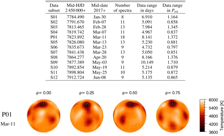
Table 2.Temporal distribution of the subsequent datasets for each individual Doppler image

Data Mid-HJD Mid-date Number Data range Data range subset 2 450 000+ 2017+ of spectra in days inProt

S01 7784.490 Jan-30 8 6.910 1.164

S02 7791.670 Feb-07 11 5.091 0.858

S03 7813.465 Feb-28 13 7.984 1.345

S04 7819.742 Mar-07 11 4.967 0.837

P01 7823.892 Mar-11 18 8.141 1.372

S05 7826.080 Mar-13 13 5.230 0.881

S06 7835.673 Mar-23 9 4.732 0.797

S07 7841.438 Mar-28 13 5.050 0.851

S08 7864.277 Apr-20 9 8.166 1.376

S09 7877.389 May-03 9 10.149 1.710

S10 7892.854 May-19 11 5.214 0.879

S11 7898.804 May-25 10 5.175 0.872

S12 7912.724 Jun-08 9 5.135 0.865

P01

Mar-11

Fig. 3.Doppler image for the PEPSI@VATT spectra. The corresponding mid-UT date is 2017-03-11, which falls just between the dates of S04 and S05 maps shown in Fig. 1.

structions as a time series we observe that subsequent maps re- veal quite similar features (cool as well as hot spots) from totally independent data. Moreover, insufficient phase sampling would introduce artificial (hot as well as cool) features at different locations from one Doppler reconstruction to the next, i.e., usually around phases where the largest phase gaps appear. However, our datasets are well sampled, and their largest gaps (usually below 0.15-0.17 phase fraction, i.e. still not very large) appear randomly along the rotation phase, therefore we do not expect such artificial hot (and cool) features at similar locations over the 13 individual Doppler reconstructions. Note especially the P01 PEPSI-map shown in Fig. 3, which falls between the S04 and S05 STELLA-maps and despite the different observing fa- cilities and independent data the recovered surface features show remarkable resemblance. This confirms not only the reliability of the reconstructed features but also the steadiness and robustness ofiMap. The polar spot seems to be the most permanent feature over the time range, while at lower latitudes the spotted surface is more variable, still, the dominant features can be tracked from one map to the next. Finally, we note that in some maps strong features are seen also below the equator, despite that Doppler imaging is less powerful when reconstructing the less visible hemisphere. We assume, however, that such a feature is most likely real when it reappears on consecutive Doppler reconstructions (see S03-S04-S05 and S10-S11), although the shape, size or contrast of these features may be loose.

The first reconstruction in the time series (S01) reveals an elongated polar feature of≈4800 K together with several lower latitude nearly circular spots of ≈4000−5000 K with typically 10^◦ diameter. The brightest feature of ≈5800 K is centered at phaseφ=0.4 at high (≈50^◦) latitude. A faint cool spot atφ=0.25

is becoming the most prominent cool feature for the next map (S02), while the hot spot as well as the other cool spots are getting less contrasted. For the next map (S03) the polar spot is getting cooler and more compact, while other cool spots are shrinking by≈30-60%. The only exception is the new cool feature at the lower hemisphere, just at the border of visibility. We note that the bright spot atφ=0.4 is permanently visible. For the next (S04) map the cool spots are becoming fainter, however, the bright spot atφ=0.4 is hotter. S05, the fifth map reveals an emerging new cool spot atφ≈0.3, while the polar spot has become more compact and contrasted. In the next map (S06) the progeny of the new spot, as well as the other cool and bright features, become smaller and/or less contrasted. This continues in S07 map, where the hot features nearly vanish. Traces of new flux emergence are seen in S08 with a new spot atφ≈0.2. Also, bright features appear again, in particular the well-known one atφ=0.4. In the next map (S09) the polar spot is getting more prominent while the newly emerged spot at φ≈0.2 fades and splits into two subspots. The high latitude bright spot atφ=0.4 is still detectible. In the tenth map (S10) a new cool spot group emerged atφ≈0.5, and is getting less contrasted and shifted towards the covered pole in the S11 map. Also, the formerly van- ishing spot around 0.2 phase appears now strengthened. This continues during our last reconstruction (S12), where the polar spot is shrinking and also displacing. Permanent rearrangements are taking place, e.g. the spot group in S11 atφ≈0.9 is getting smaller in size and cooler. Note also, that the high latitude warm (≈5600−5900 K) features are still present.

For each map the overall surface temperature is obtained by averaging the temperature values pixel by pixel over the stellar surface. However, tracing individual spots from one map to the Article number, page 6 of 18

(7)

Fig. 4.Time variation of the spot filling factor (top panel) and the integrated surface temperature (bottom panel) of IN Com derived from the time-sereies Doppler images shown in Figs. 1, 2 and 3. In the upper panel the spot filling factors are shown for the polar region and for the mid-to-low latitudes separately; see the top and the bottom curves, respectively. The different Doppler reconstructions are identified by their serial numbers.

next is hampered by the rapid spot rearrangements and/or the imperfect phase coverages. Instead, we split the surface into two parts above and below 65^◦, this way ranking the spots to be either polar or low-to-mid latitude spots. We measure the time variation of both surface partitions by deriving the spot filling factor values. In Fig. 4 we plot the time variation of the average temperature from surface integration as well as the spot filling factors.

The diagrams indicate two epochs at HJD 2 457 826 (S05) and HJD 2 457 893 (S10), when the average temperature decreased by ≈50 K, simultaneously with a small drop of the filling factor at the pole, but a significant increase of ≈40% at mid-low latitudes. According to the maps, these two events may indicate significant spot rearrangements, when new fluxes emerge. On the other hand, individual spot evolutions imply that the average spot lifetime should be of the order of a month.

3.5. Surface differential rotation

Tracking short term spot migrations is among the usual methods to study stellar surface differential rotation from Doppler imaging (Donati & Collier Cameron 1997). In this paper, we apply the programACCORD(K˝ovári et al. 2015, and references therein) and perform a time-series cross-correlation analysis

Fig. 5.Average cross-correlation map for IN Com showing anti-solar surface differential rotation. The best correlated dark regions are fitted by Gaussian curves in 5^◦bins. Gaussian peaks are indicated by dots, the corresponding Gaussian widths by horizontal lines. The best fit differential rotation law suggests an equatorial period ofPeq=5.973 d and a surface shear coefficient ofα=−0.026.

from the 12 Doppler images obtained for the STELLA observations (for the sake of data homogeneity we excluded the P01 map from this analysis). It provides 11 consecutive cross-correlation function (ccf) maps which are combined into an average correlation map. Its 2D correlation pattern is then fitted with a quadratic differential-rotation law in the usual (solar) form of Ω(β) = Ωeq(1 −αsin²β), where Ω(β) is the angular velocity at latitudeβ,Ωeqthe angular velocity at the equator, while α=(Ωeq−Ωpole)/Ωeqis the relative angular velocity difference between the equator and the pole, i.e. the surface shear coefficient.

The resulting correlation pattern for IN Com is shown in Fig. 5. It indicates anti-solar surface differential rotation, i.e., the equator rotates slower than the polar latitudes. The most well correlated dark regions are fitted with Gaussian curves in 5^◦bins. The Gaussian peaks are indicated in Fig. 5. The best fit to these peaks gaveΩeq=60.28±0.08^◦/d or an equivalent equatorial period ofPeq=5.973±0.008 d with a shear coefficient of α=−0.026±0.005. This yields a lap time of 230 d needed by the polar regions to lap the equator by one full rotation.

4. Variability of the IN Comae system

4.1. Orbital photometric modulation

Fig. 6 presents photometric data of IN Com for the past 30+

years. To support a long-period search our new photometric data are combined with the published observations from Paper I and augmented with observations from the All Sky Automated Sur- vey (ASAS) database (Pojmanski 2002). The (binned) Super- WASP data in Aller et al. (2018) could not be used due to miss- ing bandpass transformations but overlap with part of the ASAS data anyway. For the period determination, we apply the Fourier- transformation based frequency analyzer code MuFrAn (Csubry

& Kolláth 2004). In the top panel of Fig. 6, we show the best fit to the full photometric data set with a sinusoid of a period of 2639 d (≈7.2 yr), which has an uncertainty of about 200 d. The sine-wave fits well the first two well-observed cycles and does not contradict with the later, sparse data.

The photometric cycle of 2639 d is in surprising agreement with the recently proposed orbital period of 2717±63 d (Jones Article number, page 7 of 18

(8)

8.80

8.90

9.00

1985 1990 1995 2000 2005 2010 2015

V, y [mag]

5.80

5.90

6.00

6.10

46000 48000 50000 52000 54000 56000 58000

period [day]

J.D.-2400000

Fig. 6.Top: long-term photometricV andydata of IN Com. Different colors mean different sources of observations; green: data from T6 and T7 APTs, blue: observations from the Hungarian 1-m RCC telescope, red: literary data (mostly from Paper 1) which are used for seasonal period determination, grey: literary data+ASAS data which are not suitable for seasonal period determination. The sine-wave fit by black solid line represents the long-term overall brightness change with a period of 7.2 years, i.e., basically the wide binary period, see Sect. 6. Bot- tom: independent rotational period determinations for suitable seasonal datasets. See text for details.

et al. 2017) (and also with its revised value of 2689±52 d by Aller et al. 2018). Orbital phase coherence of surface activity is common in comparably short period tidally-connected RS CVn binaries, but has never been seen for such long period timescales.

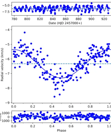
Fig. 7 shows a comparison of the orbital radial velocities with our long-term APT photometry phased with the same orbital period of 2717 days from Jones et al. (2017). Most notable is the phase coherence in the sense that the light-curve maximum coincides with a time of highest radial velocity while the light-curve minimum coincides with a time of lowest radial velocity.

4.2. Rotational photometric modulation

Seasonal short period determinations are presented in the lower panel of Fig. 6. We note that the amplitude of the rotational modulation of IN Com is generally low, typically less than 0^m.1 inV.

Therefore, seasonal rotational periods were derived only for the best quality datasets with good phase coverage and low scatter.

The average value of the seasonal periods is≈5.92 days. At this point we emphasize that any photometric period always traces the rotation period of the star at that latitude where the spot or spots occurred. Interestingly, between 1995–1999, the photometric period was increasing, while the overall brightness was decreasing. Such a simultaneity is explained by surface differential rotation that causes a shift of the dominant longitude usually populated by star spots (cf. Vida et al. 2014).

Besides, our data again demonstrate the solidity of the 5.9- day photometric period being the rotation period as opposed to,

-16 -14 -12 -10 -8 -6 -4

radial velocity [km/s]

8.80

8.85

8.90

8.95

9.00

9.05

0.0 0.2 0.4 0.6 0.8 1.0 1.2 1.4

V [mag]

orbital phase (P_orb = 2717 days)

Fig. 7.Comparing the long-term light variation with the radial velocity curve of IN Com. Top: radial velocity curve of the star taken from Jones et al. (2017); suggesting a 2717-day long orbital period. Overplotted are the radial velocities from our spectroscopic data (green circles). Bottom:

the long-termV+yphotometric observations after folding up with the orbital period.

e.g., the 1.2-day (1−f) alias. This was already done in our Paper I but then we had not had a beautiful photometric light curve that sampled the variation with high-enough time resolution. Here we present two independent, densely sampled and time-continuous APT data (Fig. 8) that proof without doubt that the 5.9-day period is indeed the correct one.

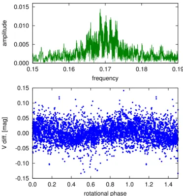
The next step is to average the individual photometric period by applying a period search to the full data set. For this, we com- bine all the available high-precisionVandydata into one single dataset and analyze it with the time-frequency analysis package MuFrAn. The resulting Fourier-amplitude spectrum is obtained for the pre-whitened data, that is the data with the long-term trend and the 2849-d period removed. The resulting amplitude spectrum is shown in the top panel of Fig. 9. Its highest peak suggests a long-term average photometric period of 5.934±0.001 d, which is very close to the average of the seasonal values. Consis- tently with the result of the differential rotation analysis in Sect. 5 this period is the apparent rotation period of the mid-latitude belt around≈35^◦where spots cause the most significant light variation. Accordingly, in the bottom panel of Fig. 9, we fold the 30+ years of photometry with this period. It shows a phase coherency that is remarkable over that period of time. Thus, for future phase calculations, we suggest to use the following equation

HJD=2,449,415.0+5.934×E, (1)

where the reference time was taken from Paper I. This is also the ephemeris that we used to phased our Doppler images in Sect. 3.

(9)

Another finding is the frequency splitting of the dominant Fourier peak at 0.17 d⁻¹. The surrounding lower amplitude peaks are typical signature of differential surface rotation of the star (see the simulations in Strassmeier & Oláh 2004). Its individual peaks mark the stellar latitudes where the spots preferentially occurred. The five most prominent peaks of the Fourier-spectrum are listed in Table 3. Assuming that these peaks are due to surface differential rotation and the lowest and highest frequencies correspond to the polar and equatorial regions (or vice versa), we estimate a surface shear parameter of∆P/P≈0.03, albeit without any presumption on its sign. Such an estimation is usually erroneous, since the origin of the photometric signals is ambigu- ous (e.g., it is not known at which stellar latitudes the signaling spots are located). Nevertheless, this value is of the same order as we found from the cross-correlation analysis in Sect. 3.5 and confirms the existence of strong differential rotation on this G5 giant.

4.3. Radial velocity modulation

The top panel of Fig. 7 also shows the STELLA SES radial velocities from 2017. Note that a systematic zero point shift of 0.503 km s⁻¹was added to this data, see Strassmeier et al. (2012) for its determination with respect to the CORAVEL system. At this point we caution that the radial velocities in the Jones et al.

(2017) paper differ in their zero point to same data re-plotted in the Aller et al. (2018) paper by≈5 km s⁻¹. A zero point correction of -2.6 km s⁻¹should be applied for the Jones et al. (2017) data to satisfactorily fit our observations.

We first remove the grossly deviant velocities by a 3-σfilter (this removed 9 data points and left 214). The remaining SES velocities of IN Com have an internal precision of typically better than 2 km s⁻¹. A Fourier analysis shows a clean peak atf ≈0.17, corresponding to a period of 5.95±0.03 d, but with an almost as strong 1− f alias. Its full amplitude is almost 2 km s⁻¹but with

8.80 8.85 8.90 8.95 9.00

50190 50195 50200 50205 50210 50215

y [mag]

J.D.-2400000 8.80

8.85 8.90 8.95 9.00

50900 50905 50910 50915 50920 50925 50930

V [mag]

J.D.-2400000

Fig. 8.Well sampled photometric modulation indicates the solidity of the 5.9-day period. Light curves were taken during April/May 1996 (top) and April 1998 (bottom) with the T7 and T6 APTs, respectively.

The light curves even show the changing amplitudes and shapes typical for star spot evolution.

0.000 0.005 0.010 0.015

0.15 0.16 0.17 0.18 0.19

amplitude

frequency

-0.15 -0.10 -0.05 0.00 0.05 0.10 0.15

0.0 0.2 0.4 0.6 0.8 1.0 1.2 1.4

V diff. [mag]

rotational phase

Fig. 9.Top: Fourier-amplitude spectrum for all the combinedVandy photometric data shown in Fig. 6. Bottom:V andydata folded with Prot=5.934 days.

an rms of the sinusoidal fit of the same order (Fig. 10). Never- theless, we can now confirm our earlier suggestion that the low- amplitude radial velocity jitter of IN Com is spot modulated. Just recently, Aller et al. (2018) arrived at the same conclusion.

5. Characteristics of the Hαprofiles

5.1. Line-profile morphology

Hαline profile variation is often associated with dynamo driven chromospheric activity, not seldom associated with a strong in- homogeneous stellar wind, coronal mass ejections and other vi- olent events like flares. The most active stars have Hαin emission. Chromospheric, transition-region and coronal activity is indeed present in the case of IN Com as amply demonstrated by, e.g. strong Caii H&K emission (see Paper 1), high-excitation UV lines like Civ(Modigliani et al. 1993) as well as strong X- ray emission (Montez et al. 2010). The overall Hαemission line profile appears permanently asymmetric which suggests intense long-lived mass motions at the upper chromosphere, giving some support to an origin related to an active binary system with mass Table 3.The five most prominent periods and their wave amplitudes from the light curve Fourier-analysis.

Frequency Amplitude Period

(1/d) (mag) (d)

0.168506 0.0143 5.934 0.171509 0.0130 5.831 0.172930 0.0130 5.783 0.169810 0.0102 5.889 0.165874 0.0085 6.029

(10)

Fig. 10.Top: rotational modulation of the disk-integrated radial velocities of IN Com. Middle: the radial velocity measurements are phase folded with the rotation period and fitted with a sinusoidal. Bottom:

residuals of the sinusoidal fit.

motions. Thus, one would expect some rotational modulation of it if it is related to IN Com in the first place.

A time series of 208 Hαline profiles from the first half of 2017 is shown in Fig. 11. A broad emission profile with an average FWHM of≈400 km s⁻¹(8.8 Å) superimposed with a central absorption reversal of width ≈150 km s⁻¹ appears consis- tently throughout the time series. The line width at continuum exceeds the expected rotational width by a factor of≈5. The rotational period and the equatorial rotational velocity give a radius of 11 R(Table 1, adopting an inclination of 45^◦from Doppler imaging). If the Hαemission is bound to the star above FWHM would then suggest an origin of at least part of the emission at an extended radius, e.g. due to a circumstellar environment of up to 3–4 R?(assuming corotation). This would mean that the overall Hαemission is composed of two parts; a chromospheric component and a circumstellar component. This has been seen and analyzed in several other (over)active stars, e.g. in UZ Librae (Zbo- ril et al. 2004), FK Comae (Ramsey et al. 1981), II Pegasi (Short et al. 1998) and others, and is not a specific issue for IN Com because it is within a planetary nebula.

All three Balmer profiles of IN Com vary slightly and con- sistently from one observation to the next while its profile morphology remains basically unaltered over our entire observing season. No rotational modulation was detected so far although there are changes seen in Hαon a decade-long scale (Aller et al.

2018). The two pseudo emission peaks frequently reverse its relative strength in our data set; once the blue emission is stronger once the red emission is stronger. At this point we note that the Hβand Hγprofiles of IN Com look vastly different than Hα.

Both are purely in absorption with an asymmetric shape but of

Fig. 11.Overplot of the HαSES spectra of IN Com from the first half of 2017. Indicated are the±300 km s⁻¹period-search limits imposed for the 2D FFT in Fig. 12.

same average width as the central Hαabsorption. We measured FWHM for Hβof 150 km s⁻¹and for Hγ of 160 km s⁻¹; however, unfortunately, Hβfalls at the edge of subsequent échelle- orders, while Hγ is significantly blended with a blue line at 4337.4 Å and therefore the S/N values for both lines are sig- nificanly lower compared with Hα; we estimate errors of 10- 15 km s⁻¹. No emission above the continuum is seen neither for Hβnor Hγ. We note that the width of the Hαabsorption reversal is in agreement with the expected rotational broadening, and so are the absorption profiles of Hβand Hγ.

5.2. Rotational modulation

To search for coherent temporal changes, we apply a 2D Fourier- periodogram to the Hαtime series. It is based on a simple fast Fourier transform (FFT) analysis to each wavelength-calibrated pixel of the Hαprofile within a velocity range of±300 km s⁻¹ around the line center (for a more detailed description of the technique see Strassmeier et al. 2014). Note that one SES CCD pixel disperses ≈0.06 Å at Hα. The resulting 2D periodogram is shown in Fig. 12. It reveals a clear and dominating peak at f = 0.169 d⁻¹ (P = 5.92±0.06 d), i.e., the expected rotation period of the giant. A second, much weaker peak is detected at 2f and is identified as its alias.

It is puzzling though that our 2D periodogram shows a gap with zero power for the 0.169 d⁻¹frequency in the red part of the line core just between zero and≈+70 km s⁻¹velocity. We have no readily explanation for this.

5.3. Line shape and width

We compare the IN Com Hα profiles with the chromospheric and transition-region models put forward by Zboril et al. (2004).

With their model 4 (Table 3 and Fig. 4 in Zboril et al. 2004), we find the overall best match for the average IN Com profile.

We note that the match is not based on a rigorous line-profile fit but only on a qualitative comparison. The enormous width of the Hαemission of > 400 km s⁻¹ had been presented as a puzzle (Aller et al. 2018) but is actually reproduced even with a normal plane-parallel atmosphere with an onset of the chromospheric temperature rise at around 5000 K at a (solar-like) mass depth of 1 g cm⁻²and the assumption of complete frequency re- Article number, page 10 of 18

(11)

-300 -200 -100 0 100 200 300

Velocity (km/s)

0.1000 0.2000 0.3000 0.4000 0.5000

Frequency (1/d)

H α

0.000 0.004 0.008 0.012 0.016 0.020 0.024 0.028 0.032 0.036 Power

Fig. 12.Two-dimensional Fourier periodogram of the time series Hα profile from Fig. 11. Spectral power is indicated in gray-scale. The plot’s horizontal range is±300 km s⁻¹ around the line core while its vertical range is from 470 d at the bottom to 2 d at the top. The dominant excess power is detected at a frequency of≈0.17, corresponding to a period of 5.92 d.

distribution (CRD), which assumes that a photon absorbed in the wings is re-emitted in the core (see Avrett & Loeser 2003). The resulting HαFWHM is of the order of 350 km s⁻¹ with a relative intensity of the emission peak of 1.2 and a 50% central self reversal. It implies an upper chromosphere with a temperature of 10,000 K and a logarithmic column density of−2.7 as well as a transition region (to the corona) with a temperature in excess of 100,000 K and a logarithmic column density of−6.

6. Summary and discussion

We have analyzed decade-long photometric and one season-long spectroscopic data of IN Com to derive more accurate stellar parameters and perform a time-series Doppler imaging study. From the long-term photometric observations we have confirmed a

≈5.973 day-long equatorial rotation period of the G-star. Also, we have provided more accurate astrophysical parameters for IN Com. Our time-series Doppler imaging study for the first

Fig. 13.Relationships between rotation and differential rotation for late- type single and binary stars. The position for IN Com is in agreement with the linear fit to (effectively) single stars, represented by the dotted line, suggesting that|α| ∝Prot[d]/200.

half of 2017 yielded 13 subsequent surface image reconstructions, which were used to estimate surface differential rotation.

We found antisolar surface rotation profile with α = −0.026 shear coefficient. This value falls within the recently proposed rotation-differential rotation relationship by K˝ovári et al. (2017), see Fig. 13. According to the plot, the linear fit for (effectively) single stars suggests|α| ∝Prot[d]/200. Moreover, the derived ab- solute surface shear of ∆Ω = 0.027[rad/d] would follow the general trend of∆Ω ∝ T_e^p_ff where p = 5.8±1.0 (see Fig. 2 in K˝ovári et al. 2017). Indeed, from the long-term photometric period variations we estimated the rate of the surface shear to be

∆P/P≈0.03, which was in agreement with the shear coefficient derived from Doppler imaging.

The G-giant star in the center of the planetary nebula shows features originating from its evolutionary history. The giant is a barium-rich star; from our spectral synthesis (see Sect. 3.1) we estimate a [Ba/Fe] ratio of 0.85±0.25, supporting the former result of 0.50±0.30 by Thévenin & Jasniewicz (1997). We redetermined [Y/Fe] and [Sr/Fe] ratios as well, confirming the overabundance of these elements in the atmosphere of IN Com. The present configuration and the overabundant s-process elements of the G-star in the binary could be explained if the precursor of the white dwarf had originally the higher mass and therefore evolved faster to the white dwarf stage, while losing mass, and afterwards the companion (now G-star) was polluted by mass- transfer or wind accretion (cf. Verbunt & Phinney 1995).

The parallel variation of the long-term light curve with the orbital phase suggests a connection between the orbital motion of the binary and the activity of the G-giant. The star is the brightest and faintest at minimum and maximum radial velocity, respectively (see Sect. 4 Fig. 7).

We note finally that, although no observational evidence has been found so far to support the existence of accreting material around the G-star, its high angular momentum, the peculiar differential rotation, the Hαbehaviour and the parallel variation of the long-term brightness with the orbital phase, may all be explained by the presence of an accretion disc tilted to the orbit.

Acknowledgements. We thank our anonymous referee for their valuable sugges- tions that have helped to improve the paper. This paper is based on data obtained with the STELLA robotic telescopes in Tenerife, an AIP facility jointly operated by AIP and IAC (https://stella.aip.de/) and by the Amadeus APT jointly Article number, page 11 of 18

(12)

operated by AIP and Fairborn Observatory in Arizona. For their continuous support, we are grateful to the ministry for research and culture of the State of Brandenburg (MWFK) and the German federal ministry for education and research (BMBF). Authors from Konkoly Observatory acknowledge support from the Austrian-Hungarian Action Foundation (OMAA). KV is grateful to the Hun- garian National Research, Development and Innovation Office for OTKA grant K-113117. KV is supported by the Bolyai János Research Scholarship of the Hungarian Academy of Sciences. The authors acknowledge the support of the GermanDeutsche Forschungsgemeinschaft, DFGthrough projects KO2320/1 and STR645/1. This work has made use of data from the European Space Agency (ESA) mission Gaia(https://www.cosmos.esa.int/gaia), processed by theGaiaData Processing and Analysis Consortium (DPAC, https://www.

cosmos.esa.int/web/gaia/dpac/consortium). Funding for the DPAC has been provided by national institutions, in particular the institutions participating in theGaiaMultilateral Agreement.

References

Aller, A., Lillo-Box, J., Vuˇckovi´c, M., et al. 2018, MNRAS, 476, 1140 Avrett, E. H. & Loeser, R. 2003, in IAU Symposium, Vol. 210, Modelling of

Stellar Atmospheres, ed. N. Piskunov, W. W. Weiss, & D. F. Gray, A21 Bisterzo, S., Gallino, R., Straniero, O., Cristallo, S., & Käppeler, F. 2011, MN-

RAS, 418, 284

Carroll, T. A., Kopf, M., & Strassmeier, K. G. 2008, A&A, 488, 781

Carroll, T. A., Strassmeier, K. G., Rice, J. B., & Künstler, A. 2012, A&A, 548, A95

Castelli, F. & Kurucz, R. L. 2004, ArXiv Astrophysics e-prints Ciardullo, R., Bond, H. E., Sipior, M. S., et al. 1999, AJ, 118, 488

Csubry, Z. & Kolláth, Z. 2004, in ESA Special Publication, Vol. 559, SOHO 14 Helio- and Asteroseismology: Towards a Golden Future, ed. D. Danesy, 396 De Marco, O., Bond, H. E., Harmer, D., & Fleming, A. J. 2004, ApJ, 602, L93 Donati, J.-F. & Collier Cameron, A. 1997, MNRAS, 291, 1

Feibelman, W. A. & Kaler, J. B. 1983, ApJ, 269, 592 Flower, P. J. 1996, ApJ, 469, 355

Gaia Collaboration, Brown, A. G. A., Vallenari, A., et al. 2018, ArXiv e-prints González Martínez-País, I., Shahbaz, T., & Casares Velázquez, J. 2014, Accre-

tion Processes in Astrophysics

Granzer, T., Reegen, P., & Strassmeier, K. G. 2001, Astronomische Nachrichten, 322, 325

Gray, D. F. 1981, ApJ, 251, 155

Gray, D. F. & Toner, C. G. 1986, ApJ, 310, 277

Guerrero, M. A. 2012, in IAU Symposium, Vol. 283, IAU Symposium, 204–210 Gustafsson, B., Edvardsson, B., Eriksson, K., et al. 2008, A&A, 486, 951 Jasniewicz, G., Acker, A., & Duquennoy, A. 1987, A&A, 180, 145

Jasniewicz, G., Acker, A., Mauron, N., Duquennoy, A., & Cuypers, J. 1994, A&A, 286, 211

Jasniewicz, G., Thevenin, F., Monier, R., & Skiff, B. A. 1996, A&A, 307, 200 Jones, D. & Boffin, H. M. J. 2017, Nature Astronomy, 1, 0117

Jones, D., Van Winckel, H., Aller, A., Exter, K., & De Marco, O. 2017, A&A, 600, L9

K˝ovári, Zs., Kriskovics, L., Künstler, A., et al. 2015, A&A, 573, A98

K˝ovári, Zs., Oláh, K., Kriskovics, L., et al. 2017, Astronomische Nachrichten, 338, 903

Kuczawska, E. & Mikolajewski, M. 1993, Acta Astron., 43, 445 Künstler, A., Carroll, T. A., & Strassmeier, K. G. 2015, A&A, 578, A101 Kupka, F., Piskunov, N., Ryabchikova, T. A., Stempels, H. C., & Weiss, W. W.

1999, A&AS, 138, 119

Lindborg, M., Hackman, T., Mantere, M. J., et al. 2014, A&A, 562, A139 Longmore, A. J. & Tritton, S. B. 1980, MNRAS, 193, 521

Malasan, H. L., Yamasaki, A., & Kondo, M. 1991, AJ, 101, 2131

Montez, Jr., R., De Marco, O., Kastner, J. H., & Chu, Y.-H. 2010, ApJ, 721, 1820 Noskova, R. I. 1989, Soviet Astronomy Letters, 15, 149

Paczy´nski, B. 1976, in IAU Symposium, Vol. 73, Structure and Evolution of Close Binary Systems, ed. P. Eggleton, S. Mitton, & J. Whelan, 75 Piskunov, N. & Valenti, J. A. 2017, A&A, 597, A16

Podsiadlowski, P. 2001, in Astronomical Society of the Pacific Conference Se- ries, Vol. 229, Evolution of Binary and Multiple Star Systems, ed. P. Podsiad- lowski, S. Rappaport, A. R. King, F. D’Antona, & L. Burderi, 239

Pojmanski, G. 2002, Acta Astron., 52, 397

Ramsey, L. W., Nations, H. L., & Barden, S. C. 1981, ApJ, 251, L101 Short, C. I., Byrne, P. B., & Panagi, P. M. 1998, A&A, 338, 191

Strassmeier, K. G., Boyd, L. J., Epand, D. H., & Granzer, T. 1997a, PASP, 109, 697

Strassmeier, K. G., Granzer, T., Weber, M., et al. 2010, Advances in Astronomy, 2010, 19

Strassmeier, K. G., Hubl, B., & Rice, J. B. 1997b, A&A, 322, 511

Strassmeier, K. G., Ilyin, I., Järvinen, A., et al. 2015, Astronomische Nachrichten, 336, 324

Strassmeier, K. G., Ilyin, I., & Steffen, M. 2018, A&A, 612, A44

Strassmeier, K. G. & Oláh, K. 2004, in ESA Special Publication, Vol. 538, Stellar Structure and Habitable Planet Finding, ed. F. Favata, S. Aigrain, & A. Wil- son, 149–161

Strassmeier, K. G., Weber, M., Granzer, T., & Järvinen, S. 2012, Astronomische Nachrichten, 333, 663

Strassmeier, K. G., Weber, M., Granzer, T., et al. 2014, Astronomische Nachrichten, 335, 904

Thévenin, F. & Jasniewicz, G. 1997, A&A, 320, 913

Tout, C. A. & Reg˝os, E. 2003, in Astronomical Society of the Pacific Conference Series, Vol. 293, 3D Stellar Evolution, ed. S. Turcotte, S. C. Keller, & R. M.

Cavallo, 100

Van Winckel, H., Jorissen, A., Exter, K., et al. 2014, A&A, 563, L10 Verbunt, F. & Phinney, E. S. 1995, A&A, 296, 709

Vida, K., Oláh, K., & Szabó, R. 2014, MNRAS, 441, 2744

Weber, M., Granzer, T., & Strassmeier, K. G. 2012, in Society of Photo-Optical Instrumentation Engineers (SPIE) Conference Series, Vol. 8451, Society of Photo-Optical Instrumentation Engineers (SPIE) Conference Series, 0 Weber, M., Granzer, T., Strassmeier, K. G., & Woche, M. 2008, in Society

of Photo-Optical Instrumentation Engineers (SPIE) Conference Series, Vol.

7019, Society of Photo-Optical Instrumentation Engineers (SPIE) Conference Series, 0

Weber, M. & Strassmeier, K. G. 2011, A&A, 531, A89

Zboril, M., Strassmeier, K. G., & Avrett, E. H. 2004, A&A, 421, 295

(13)

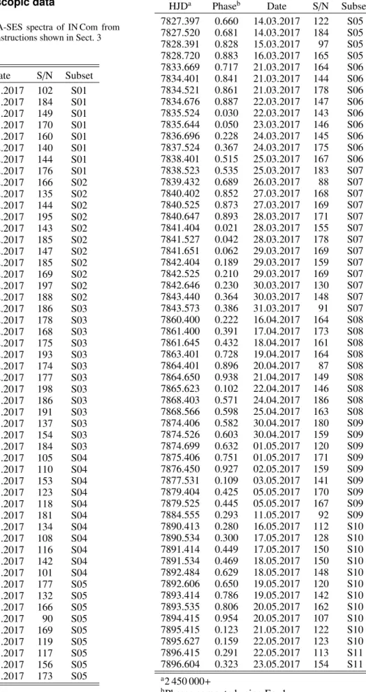
Appendix A: Log of spectroscopic data

Table A.1. Observing log of STELLA-SES spectra of IN Com from 2017 used for individual Doppler reconstructions shown in Sect. 3

HJD^a Phase^b Date S/N Subset 7780.746 0.799 27.01.2017 102 S01 7782.600 0.111 29.01.2017 184 S01 7783.521 0.266 29.01.2017 149 S01 7783.676 0.292 30.01.2017 170 S01 7784.611 0.450 31.01.2017 160 S01 7785.603 0.617 01.02.2017 140 S01 7787.503 0.937 02.02.2017 144 S01 7787.656 0.963 03.02.2017 176 S01 7788.653 0.131 04.02.2017 166 S02 7789.502 0.274 04.02.2017 135 S02 7790.496 0.442 05.02.2017 144 S02 7790.617 0.462 06.02.2017 195 S02 7791.498 0.611 06.02.2017 143 S02 7791.618 0.631 07.02.2017 185 S02 7792.498 0.779 07.02.2017 147 S02 7792.619 0.800 08.02.2017 185 S02 7793.499 0.948 08.02.2017 169 S02 7793.620 0.968 09.02.2017 197 S02 7793.744 0.989 09.02.2017 188 S02 7808.623 0.497 24.02.2017 186 S03 7811.607 0.999 27.02.2017 178 S03 7811.730 0.020 27.02.2017 168 S03 7812.494 0.149 27.02.2017 175 S03 7812.618 0.170 28.02.2017 193 S03 7812.738 0.190 28.02.2017 174 S03 7813.490 0.317 28.02.2017 177 S03 7813.612 0.337 01.03.2017 198 S03 7813.733 0.358 01.03.2017 186 S03 7815.593 0.671 03.03.2017 191 S03 7815.715 0.692 03.03.2017 137 S03 7816.486 0.822 03.03.2017 154 S03 7816.607 0.842 04.03.2017 184 S03 7817.506 0.994 04.03.2017 105 S04 7817.628 0.014 05.03.2017 110 S04 7818.495 0.160 05.03.2017 153 S04 7818.616 0.181 06.03.2017 123 S04 7819.431 0.318 06.03.2017 118 S04 7819.599 0.346 07.03.2017 181 S04 7819.720 0.367 07.03.2017 134 S04 7820.481 0.495 07.03.2017 108 S04 7821.547 0.675 09.03.2017 116 S04 7821.668 0.695 09.03.2017 142 S04 7822.473 0.831 09.03.2017 101 S04 7823.490 0.002 10.03.2017 177 S05 7823.603 0.021 11.03.2017 132 S05 7824.491 0.171 11.03.2017 166 S05 7824.694 0.205 12.03.2017 90 S05 7825.490 0.339 12.03.2017 169 S05 7825.615 0.360 13.03.2017 119 S05 7826.397 0.492 13.03.2017 117 S05 7826.521 0.513 13.03.2017 156 S05 7826.711 0.545 14.03.2017 173 S05

a2 450 000+

bPhases computed using Eq. 1.

HJD^a Phase^b Date S/N Subset 7827.397 0.660 14.03.2017 122 S05 7827.520 0.681 14.03.2017 184 S05 7828.391 0.828 15.03.2017 97 S05 7828.720 0.883 16.03.2017 165 S05 7833.669 0.717 21.03.2017 164 S06 7834.401 0.841 21.03.2017 144 S06 7834.521 0.861 21.03.2017 178 S06 7834.676 0.887 22.03.2017 147 S06 7835.524 0.030 22.03.2017 143 S06 7835.644 0.050 23.03.2017 146 S06 7836.696 0.228 24.03.2017 145 S06 7837.524 0.367 24.03.2017 175 S06 7838.401 0.515 25.03.2017 167 S06 7838.523 0.535 25.03.2017 183 S07 7839.432 0.689 26.03.2017 88 S07 7840.402 0.852 27.03.2017 168 S07 7840.525 0.873 27.03.2017 169 S07 7840.647 0.893 28.03.2017 171 S07 7841.404 0.021 28.03.2017 155 S07 7841.527 0.042 28.03.2017 178 S07 7841.651 0.062 29.03.2017 169 S07 7842.404 0.189 29.03.2017 159 S07 7842.525 0.210 29.03.2017 169 S07 7842.646 0.230 30.03.2017 130 S07 7843.440 0.364 30.03.2017 148 S07 7843.573 0.386 31.03.2017 91 S07 7860.400 0.222 16.04.2017 164 S08 7861.400 0.391 17.04.2017 173 S08 7861.645 0.432 18.04.2017 161 S08 7863.401 0.728 19.04.2017 164 S08 7864.401 0.896 20.04.2017 87 S08 7864.650 0.938 21.04.2017 149 S08 7865.623 0.102 22.04.2017 146 S08 7868.403 0.571 24.04.2017 186 S08 7868.566 0.598 25.04.2017 163 S08 7874.406 0.582 30.04.2017 180 S09 7874.526 0.603 30.04.2017 159 S09 7874.699 0.632 01.05.2017 120 S09 7875.406 0.751 01.05.2017 171 S09 7876.450 0.927 02.05.2017 159 S09 7877.531 0.109 03.05.2017 141 S09 7879.404 0.425 05.05.2017 170 S09 7879.525 0.445 05.05.2017 167 S09 7884.555 0.293 11.05.2017 92 S09 7890.413 0.280 16.05.2017 112 S10 7890.534 0.300 17.05.2017 128 S10 7891.414 0.449 17.05.2017 150 S10 7891.534 0.469 18.05.2017 150 S10 7892.484 0.629 18.05.2017 148 S10 7892.606 0.650 19.05.2017 120 S10 7893.414 0.786 19.05.2017 142 S10 7893.535 0.806 20.05.2017 162 S10 7894.415 0.954 20.05.2017 107 S10 7895.415 0.123 21.05.2017 122 S10 7895.627 0.159 22.05.2017 123 S10 7896.415 0.291 22.05.2017 113 S11 7896.604 0.323 23.05.2017 154 S11

a2 450 000+

(14)

HJD^a Phase^b Date S/N Subset 7897.601 0.491 24.05.2017 136 S11 7898.598 0.659 25.05.2017 148 S11 7899.417 0.797 25.05.2017 92 S11 7899.597 0.828 26.05.2017 140 S11 7900.613 0.999 27.05.2017 78 S11 7901.590 0.163 28.05.2017 144 S11 7910.418 0.651 05.06.2017 170 S12 7910.584 0.679 06.06.2017 127 S12 7911.418 0.820 06.06.2017 139 S12 7911.549 0.842 07.06.2017 123 S12 7912.610 0.021 08.06.2017 95 S12 7913.419 0.157 08.06.2017 171 S12 7914.419 0.325 09.06.2017 173 S12 7914.550 0.347 10.06.2017 130 S12 7915.553 0.517 11.06.2017 106 S12

a2 450 000+

(15)

Table A.2.Observing log of PEPSI@VATT spectra of IN Com from March 2017

HJD^a Phase^b Date S/NIIIc S/NVd

7819.804 0.381 07.03.2017 50 80

7819.959 0.407 07.03.2017 42 73

7820.847 0.557 08.03.2017 31 82

7820.990 0.581 08.03.2017 41 94

7821.804 0.718 09.03.2017 54 96

7821.963 0.745 09.03.2017 45 103

7822.779 0.882 10.03.2017 45 97

7822.958 0.912 10.03.2017 50 94

7823.838 0.061 11.03.2017 38 97

7824.008 0.089 11.03.2017 22 60

7824.792 0.221 12.03.2017 39 97

7824.986 0.254 12.03.2017 36 89

7825.798 0.391 13.03.2017 45 88

7826.003 0.425 13.03.2017 48 83

7826.799 0.560 14.03.2017 41 104 7826.994 0.593 14.03.2017 53 104

7827.792 0.727 15.03.2017 48 90

7827.945 0.753 15.03.2017 47 85

a2 450 000+

cSignal-to-noise ratio using CD III (blue) cross-disperser

dSignal-to-noise ratio using CD V (red) cross-disperser

(16)

S01 S02 S03

S04 S05 S06

Fig. A.1.Observed line profiles (thick black lines) and their model fits (thin red lines) for the Doppler reconstructions S01-S06 shown in Fig. 1.

The phases of the individual observations are listed on the right side of the panels.

(17)

S07 S08 S09

S10 S11 S12

Fig. A.2.Observed line profiles (thick black lines) and their model fits (thin red lines) for the Doppler reconstructions S07-S12 shown in Fig. 2.

The phases of the individual observations are listed on the right side of the panels.

(18)

Fig. A.3.Observed line profiles (thick black lines) and their model fits (thin red lines) for the Doppler reconstruction applied for the PEPSI@VATT spectra shown in Fig. 3. The phases of the individual observations are listed on the right side of the panel.