GUIDANCE AND CONTROL MULTIPLE INERTIAL SYSTEM OPERATION IN LONG TERM NAVIGATION 1 Ζ Richard R. Palmer and Donald F

M U L T I P L E I N E R T I A L S Y S T E M O P E R A T I O N IN L O N G T E R M N A V I G A T I O N

Richard R. P a l m e r and Donald F1 Ζ e McAllister Autonetics

A Division of North American Aviation, I n c0, Downey, Calif©

A B S T R A C T

T h e use of multiple s y s t e m s in long t e r m inertial navi- gation is first discussed f r o m the standpoint of reliability.

It is then s h o w n that multiple s y s t e m s are advantageous for other than reliability considerations. In particular, the use of multiple s y s t e m s in conjunction with platform rotation en- ables the continuous monitoring and rebiasing of all inertial instruments except the azimuth gyro. In this paper inertial navigation s y s t e m s are considered which are capable of inde- pendent operation and m o u n t e d so that platform orientations can be c o m p a r e d . Further, the inertial navigators are m e c h a n i z e d for local level operation (1) but the techniques presented here can be applied to other mechanizations (Z).

I N T R O D U C T I O N

Reliability and Multiple S y s t e m Operation

In the case of long t e r m operation of an inertial naviga- tor, reliability of the system and its c o m p o n e n t s is of p r i m e importance. ^ If the m e a n time to failure of a single system is

Presented at A R S Guidance, Control, and Navigation Conference, Stanford, Calif., A u g . 7-9, 1961.

^Senior R e s e a r c h Engineer.

^Senior R e s e a r c h Engineer,

^ N u m b e r s in parentheses indicate References at end of paper.

^ L o n g t e r m operation implies continuous operation of the inertial navigator for time periods on the order of w e e k s or m o n t h s .

less than the required operating period, it m a y b e c o m e expedient to have information that can be derived f r o m the operation of two or m o r e inertial navigators (multiple system operation).

In this paper it is s h o w n h o w the additional information derived f r o m multiple s y s t e m s can be used to i m p r o v e the p e r f o r m a n c e of a set of inertial navigators. This additional information is in the f o r m of differences or divergences of the outputs of two or m o r e inertial navigators. T h e p r i m a r y differences considered are position differences (from the position counters) and the attitude differences between sys- t e m s (as given by, say, gimbal angle differences). It is then s h o w n that by use of these differences and operation of the inertial platforms at different heading angles, all con- stant inertial instrument errors can be c o m p u t e d and cor- rected for, without the aid of external position, velocity, or azimuth information.

T h u s , because of the corrective and monitoring prop- erties of multiple system operation, it is s h o w n that the requirement, in long t e r m navigation, for external refer- ence information can be alleviated and the buildup of errors in the navigation system greatly reduced.

Discussion of Effects D u e to Inertial Instrument E r r o r s In a discussion of the errors associated with long t e r m inertial navigators, several coordinate f r a m e s of interest will be used, n a m e l y

Τ = true coordinate f r a m e ; a locally level set of axes erected at the actual position of the navigating v e - hicle

C = c o m p u t e r coordinate f r a m e ; a locally level f r a m e erected at the position indicated by the inertial navigator position counters

Ρ = platform coordinate f r a m e ; a coordinate f r a m e fixed to the stabilized platform

550

Each of the frames C and Ρ will, in general, be mis- aligned from the true coordinate frame Τ by some vector error angles defined by

δθ = vector error angle between the computer and true axes

φ = vector angle between the platform and true axes ψ = vector angle between the platform and computer

axes

The error angles Οθ, φ , ψ are related by the equation

Φ ^{= δθ} +Φ ^[ι]

A complete description of the error propagation in long term inertial navigation will then reside in describing the relation- ship between the error angles δθ, φ , ψ and the inertial instrument errors.

If x, y, ζ now denote axes in the north, east, and verti- cal directions, respectively, then for operation in the d a m p - ed inertial m o d e ^ (Eqs A - 1 1 , Appendix).

where

ÔV > ÔV = components of reference velocity errors

y χ

Reference velocity for damping in marine applications

is usually obtained by resolving ship's speed with respect to

the water m a s s through the platform gimbal angles.

φ » φ - level platform tilt angles

χ y

V , V ~ north and east accelerometer errors,

x y .

respectively

g = local acceleration due to gravity

Eqs. 2 state that in steady state the inertial platform will tilt through the angle φ so that the component of force sensed will exactly cancel the accelerometer error V and reference velocity error § V times the damping constant C.

The additional equations giving the position and azimuth error propagation as functions of the gyro drift rate can be derived as follows.

The angular velocity ω~ρ of the platform with respect to inertial space can be written in terms of the computed angular velocity "ÔT

and the rate of change of φ as

"ω" - ~ω~ + ώ

p c ^

The platform angular velocity is also given by the torquing rate ω

+ ψ x ω

(since the platform is misaligned from the computer axis) plus the vector gyro drift rate ε :

ω - ω + ψ χ ω _{ρ c c} ^{+ ε}

Equating Eqs. 3 and 4 gives the ψ equations

ψ ⁺ ω κ φ

c

For marine applications ω

The transfer function associated with Eq. 5 has poles at s = ±j Ω and s = 0 (for the polar component); hence, the lati- tude and azimuth errors for long term marine operations with constant gyro drift rates are oscillatory, with a period of 24 hr (the 84-min or Schüler period errors being damped, using external velocity information). The longitude error

552

for a constant polar component of gyro drift rate increases linearly with time. If the gyro drift rate is a random func- tion, the root m e a n square position and azimuth errors build up with the square root of time, since the transfer function for the ψ equations has poles on the imaginary axis. In s u m m a r y , then, it is seen that for long term damped inertial operation:

1) The level platform tilts are bounded and related to accelerometer and reference velocity error,

Z) The long term position and azimuth errors are oscillatory, with a Z4-hr periodicity.

3) Gyro drift rates cause a square root of time build up of both position and azimuth r m s error in long term oper- ation.

4) Long term operation dictates the requirement for intermittent position or azimuth fixes for realignment of the inertial system.

In the next section it will be shown how the data availa- ble from multiple system operation can be used to reduce the growth of errors in long term system operation.

M U L T I P L E S Y S T E M O P E R A T I O N Formulation of Error Differences

The various m o d e s of operation of inertial navigation systems can be characterized by the types of information used for damping purposes. Characteristic of these m o d e s is the fact that difference signals are always generated by

subtracting some quantity furnished by the system from some external reference quantity, operating on this error signal, and feeding it to various points of the system. A classification of these m o d e s follows.

1) Free inertial m o d e : no error differences used.

Z) D a m p e d inertial m o d e (or inertial m o d e with ex- ternal references): a) V

- and V

- V , the differences

' ' x rx

rv

between c o m p u t e d and reference velocity, are used to d a m p the 8 4 - m i n oscillations; b) θ - 9C and A - Λ c> ^ e differ- ences between c o m p u t e d latitude and longitude and checkpoint latitude and longitude, are used to d a m p 24-hr oscillations as well as to c o m p u t e gyro drift rate corrections; and c) φ - φ r, as furnished by a star tracker, can be used to d a m p 24-hr oscillations and correct for gyro drift rates in a stellar-monitored system.

3) Multiple s y s t e m operation: a) φ \ - φ 2> the rela- tive platform misalignment of one system with respect to the other, can be used to align one s y s t e m to another of c o m p u t e accelerometer bias error corrections by use of platform rotation; and b) δ θ ^ - 8^2» ^ e differences in indicated posi- tion between two systems, can be used to c o m p u t e gyro drift rate corrections by use of platform rotation.

In multiple inertial navigator s y s t e m s , then, the error differences available in the absence of external velocity, position, or azimuth information are

φ - φ

xl ^ x 2

Φ

Φ

se -

^,

χ 1

δ θ γ

ι

Μ

δ θ . - δθ ,

ζ 1

w h e r e the subscripts 1 and 2 refer to s y s t e m s n u m b e r 1 and 2, respectively.

T h e φ angle differences expressed in E q . 6 can be generated by observing gimbal angle differences between s y s t e m s (roll, pitch, and azimuth differences). T h e δ θ angle differences for a local level s y s t e m can be written as

δ θχ 1 " δ θχ 2 =[ Δ Λ1 ( t) " Δ A2 ( t )] C OS θ [? a]

δ % 1 - δν 2 = [θ A 9l ( t )- A 92( t )] Ν

δ θζ 1 " δθζ 2 = "[ A A! ( t )- A A2 ( t )] S i0n [7 C]

55*

w h e r e

θ, Λ = latitude and longitude, respectively

Δ θ , Δ Λ errors in indicated latitude and longitude, respectively

T h e latitude and longitude errors in E q s . 7 are given by

M H

[ec]

M

w h e r e θ , are indicated latitude and longitude for S y s t e m 1. Using E q s , 8 in E q s . 7 yields

δθ

χΐ "

^[

^{ι ω -}

^{ω ]}

^M

δ θ γ

ΐ "

2

[ ^{9 b} l

δθ

ζΐ"

-[Vt >-A

(t)] sine

Δ θ

ι

-

ι

Δ θ2 = = θ2 - θ

-

\ ^{- Λ}

Δ Α2

: - Λ

F r o m E q s . 9 it is seen that the error difference δ θ^

δ θ^ c a m be f o r m e d in t e r m s of the indicated position values only and is not a function of true position θ (t),A(t).

H e n c e , all six differences in E qe 6 can be f o r m e d without the aid of any external information.

U s e of E r r o r Differences With Platform Rotation F o r Correction of the Inertial Instruments

1. Correction of A c c e l e r o m e t e r E r r o r s in Multiple S y s t e m s Using Platform Rotation

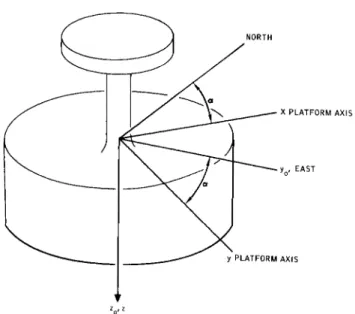
Operation of the inertial platform with an arbitrary azimuth orientation α about the ζ axis, as in Fig. 1, m u s t n o w be considered. In Fig. 1, χ , ν , ζ are in the north,

ο ο ο

east, and local vertical directions, respectively. T h e physi- cal platform axes x, y, ζ are obtained by a rotation about the vertical through the angle a, as shown. T o accomplish this rotation with ease, the gimbal order in going f r o m the plat- f o r m to the ship m u s t be azimuth first (about z) and then pitch or roll.

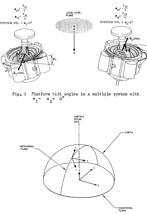
Fig, 2 depicts the steady state level tilts of two inertial navigators operated with = = 0 ° , that is, in north-

pointing orientation* F r o m E q s . 2 the 0 differences between s y s t e m s are given by

[ * x l- * x d Vyl

-

0 g

= v

- ν

0° _g

If platform 2 is n o w rotated by 180° with respect to platform 1 and allowed to level up, the φ differences w be

^ x l ' <^x2) 180.°=

yl y 2

(Φ . - Φ

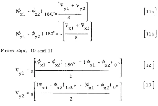
F r o m E q s . 10 and 11

^xl ^ x 2

y2

xl x 2 180 xl x 2 0

10a]

10b]

11

11a]

lib]

12

13

556

yl y2'

v

V

x 2 -

< V V ¹⁸⁰ - < W

[ 1 4 ]

H

The computed accelerometer bias errors (Eqs. 12 and 15) can now be subtracted from the output of the correspond- ing accelerometer, thus correcting for the level misalign- ment of both platforms. The implicit assumption that

the bias errors do not change during the measurement period should be noted.

2. Correction for Level Gyro Drift Rates in Multiple Systems The coordinate frame p, y, h shown in Fig. 3, in which x, y, ζ are local level axes will be considered. The axes p, y, h are defined as follows: ρ is along Earth's polar axis, y is identical to the east-pointing axis in local level axes, and h completes the triad. F r o m this figure it is seen that the angle between χ and ρ is simply the latitude of the

system. Hence

€ cos θ + ί sin θ P h

e - e

y y

* = * cos θ -

sin θ ζ h ρ

[ 1 6 a ]

[ 1 6 b ]

[ l 6 c ]

Similarly

φ -φ cos θ +Φ

^{sin θ}

χ ^ ρ h

y y t " » ]

φ -φΛ cos θ - ψ sin θ

ζ η ρ [ H e ]

Writing the ψ E q s . 5 in p, y, h coordinates and integrating, the constant gyro drift rates can be solved for as functions of ψ:

Ρ t

Ω sin Ω t

<A

ir IT

[18a]

ί -

_ Ω sin Ω t y 2(1 - cos ΩΟ

Ω

V t > - *

( 0 ) J + 2 ^ <t)+* ^{(0 )J}

Ψ

^

(ο) ^<A

+<A

(o)

It will n o w be a s s u m e d that there are available two inertial navigators operating in either the free or d a m p e d inertial m o d e . It has been seen h o w the difference φ^ - φ^

and θθ^ - between S y s t e m s 1 and 2 can be f o r m e d . T h e n the φ differences can be f o r m e d f r o m E q^e 1:

Δψ =Φ^ι-ψ^ζ =

(Φ

- Φ

) - (δθ

- δ β

)

H e n c e , using E q s . 18 and 19

Αφ (t) - Αφ (0) Ρ ?

558

ι

_ Ω sin Ω t

hi "fh Z " 2(1 - cosftt)

A ^

( t ) - A«A

(0) Ω

+ 2 Δι/^(ΐ) + Αφ (0)

Ω

cy l " 2(1 - c o s ü t )

Ω

~ 2

ΔιΑ (t) -

[20b]

[ 2 0 c]

w h e r e the ^differences in E q s . 20 are given by

\(t)

- ^ ( t ) Φ ,(t) - Φ ,(t)

zl z2 sin θ

Φ

( 0 - Φ

( 0

θ

Αφ

(t) =

y A«A^h(t)

Φ

( 0 - Φ

( 0

e^t) - e

(t)

sin θ

^

(t)-*

(t)

θ * (t) - θ _(t)|cos θ

ζ 1 ζ2

ι»]

If E q s . 21 and 23 are f o r m e d f r o m the differences in s y s t e m outputs between two inertial navigators with * a = 0 ° , the differences in gyro drift rate can be c o m p u t e d f r o m E q s , 16 and 20, as illustrated in Fig, 4,

fx l -fx 2 = ( fp l -fp 2) C O S 9+(fh l -fh 2} S i n9

x 0° [24a]

€ . - ( - = (Δί )

yi

^o

[24b]

zl z2 1 hi h 2

= (Δ< ) ζ 0°

Κ , -

, J cos θ - (e - < ) sin θ

[24c]

If S y s t e m 2 is n o w rotated so that the χ axis is south

= 180°), the following can be c o m p u t e d observing ΔΨ at two discrete times:

e + €

xl x2

yl y2

(Δί

χ

( A

V

£z l " (z2 = (Δί )

ζ' 180°

[25a]

[25b]

[25c]

F r o m E q s . 24 and 25 level gyro drift rates can n o w be c o m - puted for both systems:

xl

x2

yz

(Δί

Λο

^<

^χ>ΐ80°

: (Δ ίχ) 1 8 0 ° - ( Δ ίχ) Q O:

1*

I

(Δί ) ο + (Δί )

y y 180° [28

2 -

( A

V

V

36ο

After the multiple s y s t e m biasing run is completed, E q s . 2 6 and 2 9 can be applied to the gyros as gyro bias corrections.

It is to be noted that neither the accelerometer nor gyro biasing s c h e m e presented requires external position.

S U M M A R Y

In the previous section it w a s s h o w n h o w gyro and accel- e r o m e t e r bias corrections can be generated by the use of data internal to the operation of two or m o r e inertial navigators.

B y applying these corrections, the effective inertial instru- m e n t errors are reduced w h e n the correlation times of the instrument errors are longer than the m e a s u r e m e n t periods. B y these procedures, then,, the long t e r m error buildup characteristic of long t e r m navigation s y s t e m s can be decreased.

Multiple s y s t e m operation, then, can be used in con- junction with periodic checkpoint information for bounding position, attitude, and azimuth errors to acceptable values for long time periods. This is in addition to the overall gain in reliability afforded by two or m o r e inertial navigators.

A P P E N D I X : D E R I V A T I O N O F S T E A D Y S T A T E E X P R E S S I O N S F O R L E V E L P L A T F O R M T I L T A N G L E S IN T H E D A M P E D I N E R T I A L M O D E

T h e position error vector can be written as

w h e r e R denotes the position vector as m e a s u r e d f r o m the center of Earth to the true position, and O R is the position error in the c o m p u t e d position. T h e n the position error equation for operation in the d a m p e d inertial m o d e is (where derivatives are taken with respect to the true coordinate s y s t e m )

SR ^{= δθ χ R}

O R ^+·λ) O R + 2 Ω χ O R

ο ζ

= -co2

φ

w h e r e

Ω Ω

Ζ

V

c

δν

Schuler angular frequency (4

458 rad/hr) Earth rate (15 deg/hr)

= vertical component of Earth rate (Ω = -fisin Θ)

= accelerometer bias error vector velocity damping constant (c = Ζζ ω , where ζ = damping ratio)

reference velocity error vector

The φ equations are given by

- 7 - + ω

χ

φ

c ^

A-3

where

e = gyro drift rate

ω^(Ζ

» computed angular velocity ( OJ

moving vehicles)

Eq. A-Ζ can be rewritten in component form in the frequency domain as

(s + Cs + Ζ Ζ

) - ΖΩ s

ο

ΖΩ s (s + Cs + Ζ Ζ

ζ

ο

ÔR (s) χ

ÔR (s) y

Q

(s)

Q

(s)

where Q (s) and Q (s) are the transforms of the χ and y x y

components of the driving functions of Eq. A - 2 .

362

Eqs. A

OR (s)

(s

+ Cs

_o ) Q (s) + 2 Ω s Q _{x z y} (s)

2 2 2 2 ? (s + Cs +

4Ω s

ο ζ

Α-5

ÔR (s) y

(s

+ Cs + ω

} Q (s) -

(s) ο y ζ x 2 2 2 2 2 (s + Cs

) + 4 Ω s

ο z

A-6

The poles of the transfer functions in Eqs* A-5 and A-6 are in the left half-plane for C > 0 . Hence, the position error response for driving functions whose frequency is m u c h less than the Schüler frequency

^ and for constant driving functions is

OR xSS

Q (t)

χ A - 7

OR ySS

Q (t)

y A

or

2 Τ -

ω ψ _Χ

R + ν + c sv

8R

ω

' A - 9 J

Using the identity φ = Φ - δ θ in Eqs, A -9 and A-l

φ ^{X R = -}

^{— + C}

ω ω

ο ο

[ Α- , ο ]

Expanding equation A -1 0 in c o m p o n e n t f o r m , E q s . A - l l a and A - l i b w i l l r e s u l t

Φ

a "

o A - l l a ]

Φ

δγ

a ω ο A - l l b

REFERENCES

1 Pinson, J«C., "Inertial guidance for cause vehicles,^,f Autonetics publication £ï>2-A-6, Downey, Calife, ppo

2 McMurray, L^cRo, "Alignment of an inertial autonavigator,"

ARS J. 31, 356-360 (1961).

Fig. 1 Operation of an inertial navigation system with arbitrary azimuth angle

364

Fig

2 Platform tilt angles in a multiple system with

E A R T H ' S P O L A R A X I S

M E R I D I O N A L P L A N E

E A R T H

P L A N E

Figo 3 Platform and Earth-fixed coordinate axes