MINIMAL ENERGY POINT SYSTEMS ON THE UNIT CIRCLE AND
1
THE REAL LINE
2
MARCELL GA ´AL∗, B ´ELA NAGY†, ZSUZSANNA NAGY-CSIHA‡, AND SZIL ´ARD 3
GY. R ´EV ´ESZ∗ 4
Abstract.
5
In this paper, we investigate discrete logarithmic energy problems in the unit circle. We study 6
the equilibrium configuration ofnelectrons andn−1 pairs of external protons of charge +1/2. It 7
is shown that all the critical points of the discrete logarithmic energy are global minima, and they 8
are the solutions of certain equations involving Blaschke products. As a nontrivial application, we 9
refine a recent result of Simanek, namely, we prove that any configuration ofnelectrons in the unit 10
circle is in stable equilibrium (that is, they are not just critical points but are of minimal energy) 11
with respect to an external field generated byn−1 pairs of protons.
12
Key words. Blaschke product, electrostatic equilibrium, potential theory, external fields 13
AMS subject classifications. 31C20, 30J10, 78A30 14
1. Introduction and preliminaries. The motivation of this work comes from
15
certain equilibrium questions which, in turn, have roots in rational orthogonal sys-
16
tems. Exploring the connection between critical points of orthogonal polynomials and
17
equilibrium points goes back to Stieltjes. For more on this connection, see, e.g., [9],
18
[10] and the references therein.
19
Rational orthogonal systems are widely used on the area of signal processing,
20
and also on the field of system and control theory. These systems consist of rational
21
functions with poles located outside the closed unit disk. A wide class of rational
22
orthogonal systems is the so-called Malmquist-Takenaka system from which one can
23
recover the usual trigonometric system, the Laguerre system and the Kautz system
24
as well. In earlier works, in analogy with the discrete Fourier transform, a discretized
25
version of the Malmquist-Takenaka system was introduced.
26
In signal processing and system identification (e.g. mechanical systems related
27
to control theory) the rational orthogonal bases and Malmquist–Takenaka systems
28
(e.g. discrete Laguerre and Kautz systems) are more efficient than the trigonometric
29
system in the determination of the transfer functions. There are lots of results in this
30
field, see e.g. [3] and the references therein, or [13] and [7].
31
In connection with potential theory, it was studied (e.g. in [14]) whether the
32
discretization nodes satisfy certain equilibrium conditions, namely, whether they arise
33
from critical points of a logarithmic potential energy. Such discretizations appear
34
naturally, see e.g. [1] by Bultheel et al or [5] by Golinskii. The question whether the
35
critical points are minima was proposed by Pap and Schipp [14, 15]. In this paper,
36
we follow this line of research. After this introduction and statements of results,
37
we study on the unit circle a quite general logarithmic energy which is determined
38
by a signed measure, and prove that after inverse Cayley transform the transformed
39
energy on the real line differs only in an additive constant. Next using a recent result
40
of Semmler and Wegert [16] we give an affirmative answer to the question posed by
41
∗Alfr´ed R´enyi Institute of Mathematics, Budapest, Hungary (gaal.marcell@renyi.hu, revesz.szilard@renyi.hu).
†MTA-SZTE Analysis and Stochastics Research Group, University of Szeged, Szeged, Hungary (nbela@math.u-szeged.hu).
‡Institute of Mathematics and Informatics, University of P´ecs, (ncszsu@gamma.ttk.pte.hu) and Department of Numerical Analysis, E¨otv¨os Lor´and University, Budapest, Hungary .
1
Pap and Schipp concerning the critical points. Finally, as an application, we present
42
a refinement of a result of Simanek [18].
43
First let us start with some notation and essential background material. We
44
use the standard notations D := {z ∈ C : |z| < 1}, ∂D := {z ∈ C : |z| = 1},
45
D∗ :={z∈C: |z|>1},T:=R/2πZandζ∗ := 1/ζ (ζ 6= 0). We also use Blaschke
46
products, defined fora1, . . . , an∈Dandχ,|χ|= 1 as
47
(1.1) B(z) :=χ
n
Y
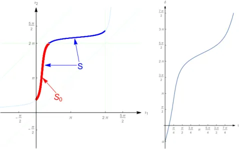
k=1
z−ak
1−akz.
48
In particular, when the leading coefficient χ = 1, B(z) is called monic Blaschke
49
product.
50
We assumeB0(0)6= 0. In this case the well-known Walsh’ Blaschke theorem (see
51
for instance [17], p. 377) says thatB0(z) = 0 has 2n−2 (not necessarily different)
52
solutions, wheren−1 of them (counted with multiplicites) are in the unit disk, and
53
ifζ∈D\ {0}satisfies B0(ζ) = 0, thenζ∗:= 1/ζ is also a critical point,B0(ζ∗) = 0,
54
with the same multiplicity asζ. It also follows that then B0|∂D6= 0.
55
Next, we investigate the structure of solutions of the equation
56
(1.2) B(eit) =eiδ,
57
whereB(.) is a Blaschke product. It is standard to see that=logB(eit) can be defined
58
continuously and it is strictly increasing on [0,2π] from
59
α:==logB(1) = argB(1), α∈[−π, π)
60
to α+ 2nπ, see, e.g. [17], pp. 373-374. Therefore (1.2) has n different solutions in
61
t∈[0,2π) for any δ∈R. Hence it is logical to considern-tuples of different solutions
62
as solution vectors for (1.2).
63
Now, we are to reduce different types of symmetries among the solution vectors
64
step-by-step. For givenδ∈R, consider
65
(1.3)
(τ1, . . . , τn)∈Rn:B eiτj
=eiδ, j= 1, . . . , n .
66
We can restrict our attention to the reduced setτ1≤τ2≤. . .≤τn ≤τ1+ 2πwithout
67
loss of generality, for picking any τ1 we can normalize mod 2π and then order the
68
remainingτj. Actually, since theτj are different, all such solutions of (1.2) belong to
69
the open set
70
(1.4) A:=
(τ1, τ2, . . . , τn)∈Rn : τ1< τ2< . . . < τn < τ1+ 2π .
71
It is a standard step (see [17] loc. cit.) that one can define the functions δ7→τj(δ)
72
such that they are continuously differentiable, strictly increasing, andτ1(δ)< . . . <
73
τn(δ) < τ1(δ) + 2π for all δ ∈ R, whileB(exp(iτj(δ))) = exp(iδ) j = 1, . . . , n. As
74
B(ei0) =eiα, we have 0∈ {τ1(α), τ2(α), . . . , τn(α)}. By relabelling again, if necessary,
75
we may assume that
76
(1.5) τ1(α) = 0.
77
Hence T(δ) := τ1(δ), . . . , τn(δ)
can be viewed as a smooth arc lying in A ⊂ Rn.
78
Moreover, the graphSR:={T(δ) : δ∈R}contains all the solutions of (1.2) fromA,
79
that is, ift:= (t1, . . . , tn)∈A and λ∈Rare such that B(exp(itj)) = exp(iλ), j =
80
2
1, . . . , n hold, then there existsδ∈Rsuch that t=T(δ). Furthermore, exp iτj(δ+
81
2nπ)
= exp iτj(δ)
forj= 1,2, . . . , n, δ∈R. We introduce the set
82
(1.6) S0:=SR∩[0,2π)n={T(δ) : δ∈[α, α+ 2π)}
83
where we used (1.5). We call the set
84
(1.7) S:={T(δ) :δ∈[α, α+ 2nπ)}
85
thesolution curve. Note that
86
S =SR∩Q, where
87
Q:= [0,2π)×[τ2(α), τ2(α) + 2π)×. . .×[τn(α), τn(α) + 2π)
8889
where we also used (1.5), so [τ1(α), τ1(α) + 2π) = [0,2π). Geometrically, S can be
90
obtained fromS0 with reflections and translations, whileSRcan be obtained fromS
91
with translations only. Another useful property ofS is that for eachβ∈[0,2π) there
92
is exactly oneδ∈[α, α+ 2nπ) such thatτ1(δ) =β.
93
-π 2
π 2π 5π
2 τ1
-π 2 π 2π 5π 2 τ2
S0 S
π 4
π 2
3π 4
π 5π 4
3π 2
7π 4
t
α π 2 π 3π 2 2π 5π 2 3π 7π 2 δ
Figure 1.Left: solution curveSof the monic Blaschke product with zeros at1/2and(1 +i)/2, 0≤τ1< τ2<2π,B(eiτ1) =B(eiτ2) =eiδ,α≤δ≤α+ 2π, whereα=−π/2now. Right: argument of the same monic Blaschke product,δ= argB(eit).
These are depicted on the left half of Figure1whereS0 is the thick arc and it is
94
continued above with another arc. These two arcs together formS and describe the
95
motions ofτ1, τ2together as exp(iδ) goes around the unit circle twice (δ grows from
96
αto α+ 4π). Extending these two arcs with the very thin arcs, we obtain SR, the
97
full solution curve.
98
Now we recall the question raised by Pap and Schipp in [15]. Consider the pairs
99
of protons, each of charge +1/2, at ζ1, ζ1∗, . . . , ζn−1, ζn−1∗ as the critical points of a
100
(monic) Blaschke product of degreen, and the (doubled) discrete energy of electrons
101
restricted to the unit circle
102
(1.8) W(w1, . . . , wn) :=
n−1
X
k=1 n
X
j=1
log|(wj−ζk)(wj−ζk∗)| −2 X
1≤j<k≤n
log|wj−wk|
103
3
where |w1| = 1, . . ., |wn| = 1. The set SR connected to the same monic Blaschke
104
product yields critical configurations of electrons for each fixedδ(which corresponds to
105
fixing one of the electrons), according to e.g. [15]. In other words, fora1, . . . , an∈D,
106
using the monic Blaschke product with zeros ata1, . . . , an one can construct pairs of
107
protons as solutions of B0(z) = 0, and, for any givenδ ∈[0,2π), the corresponding
108
configuration of electrons as all solutions of B(z) = eiδ. Then according to the
109
result of Pap and Schipp, Theorem 4 from [15], these configurations of electrons are
110
critical points ofW. The question posed on p. 476 of [15] is then: Are these critical
111
points (local) minima of the restricted energy function Wf where Wf(τ1, . . . , τn) :=
112
W eiτ1, . . . , eiτn
, τ1. . . , τn∈R?
113
We give a positive answer to this question in general. Note that two special cases
114
were solved in [15] with different methods. Our answer is the following. There are
115
no other critical points on the unit circle (where the tangential gradient vanishes).
116
Moreover, all the points on the set SR are global minimum points of the restricted
117
energy functionWf.
118
Theorem 1.1. Leta1, . . . , an∈DandB(z)be the monic Blaschke product (1.1)
119
with zeros at a1, . . . , an. Assuming B0(0) 6= 0, list up the critical points of B as
120
ζ1, . . . , ζn−1∈D\ {0}andζ1∗, . . . , ζn−1∗ ∈D∗.
121
Then the tangential gradient ofW vanishes on the points corresponding to the set
122
A∩Qdefined in (1.4)exactly on the setS.
123
More precisely, on A ∩Q, it holds that ∇Wf(τ1, . . . , τn) = 0 if and only if
124
(τ1, . . . , τn) =T(δ) for someδ∈[α, α+ 2nπ).
125
Furthermore, all points of SR are global minimum points ofWf.
126
Let us recall here a recent result of Simanek [18, Theorem 2.1]. Briefly, he estab-
127
lished that for any configuration of electrons on the unit circle, there is an external
128
field (collection of protons) such that the electrons are in electrostatic equilibrium
129
(that is, the gradient of the energy is zero). We are going to refine this result by de-
130
termining the number of pairs of protons and their locations using the solution curve
131
defined in (1.7).
132
For the following we need some more results on Blaschke products. Namely for
133
givenz1, z2, . . . , zn∈C,|zj|= 1,zj6=zk (j6=k), we need to find a Blaschke product
134
B(.) of degreem, such that
135
(1.9) B(zj) =χ
m
Y
k=1
zj−ak
1−akzj = 1, j= 1,2, . . . , n.
136
The first result of this kind was established by Cantor and Phelps in [2] (for somem)
137
and the stronger form with degree m ≤n−1 was given by Jones and Ruscheweyh
138
in [11], see also a paper by Hjelle [8]. By using the results of Jones and Ruscheweyh,
139
Hjelle showed that there is a Blaschke product B(z) of degree m = n such that
140
(1.9) holds, see [8], p. 44. We will use this particular Blaschke product B(z) =
141
B(z1, z2, . . . , zn;z) corresponding toz1, z2, . . . , zn. Note that Hjelle’s Blaschke prod-
142
uct is not unique, since there is an extra iterpolation condition. Observe that the
143
extra interpolation condition can be chosen so thatB0(0)6= 0 is satisfied.
144
Theorem 1.2. For distinctz1, . . . , zn ∈∂D fix a Blaschke productB(z) so that
145
(1.9)holds with m=n andB0(0)6= 0. Denote the critical points ofB(z)in the unit
146
disk byζ1, ζ2, . . . , ζn−1.
147
Then the (doubled) energy functionW(w1, . . . , wn), constructed by means of these
148
pointsζ1, ζ2, . . . , ζn−1according to(1.8), has critical point at(w1, . . . , wn) = (z1, . . . , zn)
149
4
(even regarded as a point ofCn).
150
Moreover, on (∂D)n,W|(∂D)n has global minimum at(z1, . . . , zn).
151
2. Some basic propositions. Recall that it was given in (1.8) the discrete
152
energy of an electron configurationw1, . . . , wn ∈C (with charges−1) in presence of
153
an external field generated by pairs of fixed protonsζ1, ζ1∗, ζ2, ζ2∗, . . . , ζn−1, ζn−1∗ (with
154
charges +1/2 each), whereζ1, . . . , ζn−1 ∈D. Note that actually W is the double of
155
the physical energy of the system (see also [12], p. 22 where they use this form of
156
discrete energy). We will see later on why it is more convenient to use this ”doubled
157
energy”.
158
Sometimes the following exceptional set will be excluded:
159 160
(2.1) E:=
(w1, . . . , wn, ζ1, . . . , ζn−1)∈Cn×Dn−1:
161
ζj= 0 for somej orwj=wk for somej6=k,
162
or ζj =wk orζj∗=wk for some j, k .
163164
This is a closed set with empty interior. Geometrically, this set covers the cases when
165
some of the protons are at the origin, some of the electrons are at the same position
166
or a proton and an electron are at the same position. Let us remark also thatW =
167
W(w1, . . . , wn) is locally the real part of a holomorphic function whenζ1, . . . , ζn−1are
168
fixed andW is considered on (w1, . . . , wn)∈Cnsuch that (w1, . . . , wn, ζ1, . . . , ζn−1)6∈
169
E.
170
This energy can be generalized substantially. Let µbe a signed measure on C.
171
We define the (doubled) energy in this case as
172
Wµ,1:= 2
n
X
k=1
Z
C
log|wk−ζ|dµ(ζ), Wµ,2:= X
l6=k 1≤l,k≤n
log|wl−wk|, and
173
Wµ(w1, . . . , wn) :=Wµ,1−Wµ,2. (2.2)
174175
Note that in (1.8) we sum over alll < kpairs and there is an extra factor 2. In (2.2),
176
the sum is over alll6=kpairs. Later this second, symmetric expression will be more
177
convenient.
178
Here, it may happen that Wµ,1 or Wµ,2 becomes infinity, so we again introduce
179
the exceptional set as follows:
180 181
(2.3) Eµ:={(w1, . . . , wn)∈Cn : wj=wk for somej6=k
182
or Z
C
|log|wj−ζ||d|µ|(ζ) = +∞for somej}.
183 184
Note that finiteness of this latter integral is equivalent to the finiteness of the potentials
185
ofµ+andµ−atwj whereµ+,µ−are the positive and negative parts ofµrespectively.
186
Observe that if (w1, . . . , wn)6∈Eµ, thenWµ,1 andWµ,2are finite, and so isWµ.
187
An important tool in our investigations is the Cayley transform and its inverse.
188
Basically, it is just a transformation between a half-plane and the unit disk, though
189
there is no widely accepted, standard form of it. We use the following form, which we
190
call inverse Cayley transform
191
C(z) =Cθ(z) :=i1 +ze−iθ 1−ze−iθ
192
5
where θ ∈ R will be specified later. It is standard to verify that C(z) maps the
193
unit disk onto the upper half-plane,Cθ(eiθ) =∞, andC(.) maps bijectively the unit
194
circle (excludingeiθ) to the real axis. Furthermore,Cθ(eit) is continuous and strictly
195
increasing fromt=θ tot =θ+ 2π, Cθ(eit)→ −∞ ast →θ+ 0,Cθ(eit)→+∞as
196
t→θ+ 2π−0. It is easy to see thatC(z∗) =C(z) andC0(z)6= 0 (ifz6=eiθ). Later
197
we will use the Cayley transform too:
198
Cθ−1(u) =eiθu−i u+i.
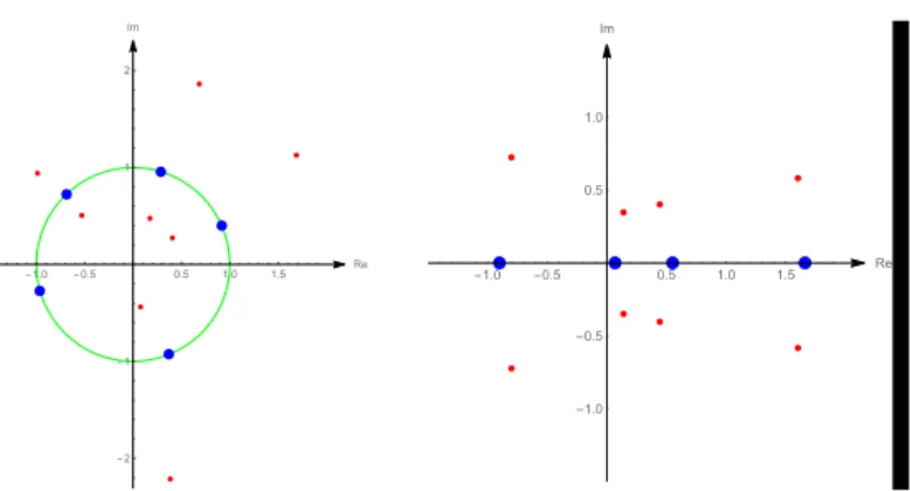
199
Mapping the electrons and protons byCθ, we definetjwithtj=Cθ(wj). We also
200
write ξj := Cθ(ζj) and accordingly, ξj = Cθ(ζj∗) and investigate the following new
201
discrete energy:
202
(2.4) V(t1, . . . , tn) :=
n−1
X
k=1 n
X
j=1
log|(tj−ξk)(tj−ξk)| −2 X
1≤j<k≤n
log|tj−tk|.
203
We also define the (doubled) discrete energy on the real line when the external
204
field is determined by a signed measureν:
205
Vν,1:= 2
n
X
k=1
Z
C
log|tk−ξ|dν(ξ), Vν,2:= X
l6=k 1≤l,k≤n
log|tl−tk|and
206
Vν(t1, . . . , tn) :=Vν,1−Vν,2. (2.5)
207208
We introduce again the exceptional set corresponding toν as follows:
209 210
Eν :={(t1, . . . , tn)∈Cn : tj =tk for some j6=k
211
or Z
C
|log|tj−ξ||d|ν|(ξ) = +∞for somej}.
212 213
The next result gives a somewhat surprising connection how the inverse Cayley
214
transform carries over energy. Actually, there is a cancellation in the background
215
which makes it work.
216
Proposition 2.1. Fix θ ∈R and let µ be a signed measure on C with compact
217
support such that µ({0}) = 0, µ(C) = n−1. Write ν :=µ◦Cθ−1, that is, ν(B) =
218
µ(Cθ−1(B))for every Borel set B.
219
Assume thatw1, . . . , wn∈Cand(w1, . . . , wn)6∈Eµ and
220
(2.6)
Z
C
log|ζ−eiθ|dµ(ζ)is finite.
221
Then with t1, . . . , tn ∈ C where tj = Cθ(wj), we know that (t1, . . . , tn) 6∈ Eν,
222
Wµ(w1, . . . , wn) andVν(t1, . . . , tn) are finite and we can write
223
(2.7) Wµ(w1, . . . , wn) =Vν(t1, . . . , tn) +c
224
wherec is a finite constant, namely
225
(2.8) c=n(n−1) log(2)−2n Z
C
log|ξ+i|dν(ξ).
226
6
Proof. It is straightforward to verify that (t1, t2, . . . , tn)6∈Eν. Furthermore,
227 228
Z
C
log|ξ+i|dν(ξ) = Z
C
log|Cθ(ζ) +i|dµ(ζ) = Z
C
log i
1 +1 +ζe−iθ 1−ζeiθ
dµ(ζ)
229
= Z
C
log(2)−log|ζ−eiθ|dµ(ζ),
230 231
so (2.6) is equivalent to
232
(2.9)
Z
C
log|ξ+i|dν(ξ) is finite.
233
Note that this entails the finiteness ofc defined in (2.8).
234
With the notation of the Proposition,
235 236
(2.10) Wµ(w1, . . . , wn)−Vν(t1, . . . , tn) = 2
n
X
k=1
Z
C
log|wk−ζ|dµ(ζ)
237
− X
j6=k 1≤j,k≤n
log|wj−wk| −2
n
X
k=1
Z
C
log|tk−ξ|dν(ξ) + X
j6=k 1≤j,k≤n
log|tj−tk|
238 239
where we investigate the difference of the integrals and difference of the sums sepa-
240
rately. So we write
241 242
Z
C
log|wk−ζ|dµ(ζ)− Z
C
log|tk−ξ|dν(ξ)
243
= Z
C
log|Cθ−1(tk)−Cθ−1(ξ)|dν(ξ)− Z
C
log|tk−ξ|dν(ξ)
244
= Z
C
log
eiθ
tk−i
tk+i−ξ−i ξ+i
−log|tk−ξ|dν(ξ)
245
= Z
C
log(2) + log
1 (tk+i)(ξ+i)
dν(ξ)
246
= Z
C
−log|ξ+i|dν(ξ) + (log(2)−log|tk+i|)ν(C),
247 248
where this last integral exists, by assumption (2.9). Similarly,
249 250
log|tj−tk| −log|wj−wk|= log|tj−tk| −log|Cθ−1(tj)−Cθ−1(tk)|
251
= log|tj−tk| −log
eiθ
tj−i tj+i
−eiθ
tk−i tk+i
252
=−log(2) + log|tj+i|+ log|tk+i|.
253254
7
Substituting into (2.10), we get
255
Wµ(w1, . . . , wn)−Vν(t1, . . . , tn)
256
= 2
n
X
k=1
Z
C
−log|ξ+i|dν(ξ) + (log(2)−log|tk+i|)ν(C)
257
+ X
j6=k 1≤j,k≤n
(−log(2) + log|tj+i|+ log|tk+i|)
258
=−2ν(C)
n
X
k=1
log|tk+i|+ 2nν(C) log(2)−2n Z
C
log|ξ+i|dν(ξ)
259
−n(n−1) log(2) + 2(n−1)
n
X
k=1
log|tk+i|
260
=n(n−1) log(2)−2n Z
C
log|ξ+i|dν(ξ),
261 262
where we used thatν(C) =n−1.
263
Remark 2.2. Sinceµhas compact support,suppν is disjoint from−i, moreover,
264
their distance is positive. Hence the logarithm in the integral in (2.8)is bounded from
265
below. It is not necessarily bounded from above, but we assume (2.9)directly. Instead
266
of supposing (2.9), we may suppose that µ and θ (from Cayley transform) are such
267
that suppµandeiθ are of positive distances from each other. This would ensure that
268
suppν remains bounded entailing that the logarithm in the integral in (2.9)is bounded
269
from above. In other words, ifsuppµis compact and eiθ6∈suppµ, then (2.9)holds.
270
We note that this Proposition2.1extends the result of Theorem 6 in Pap, Schipp
271
[15] that we allow arbitrary signed external fields in place of discrete protons located
272
symmetrically with respect to the unit circle.
273
Proposition 2.3. We maintain the assumptions and notations of Proposition
274
2.1. Let`∈ {1, . . . , n} and letwj,j 6=` be fixed.
275
Assume that
276
(2.11) eiθ 6∈suppµ
277
and assume further that replacing w` by eiθ, we have
278
(2.12) (w1, . . . , eiθ, . . . , wn)6∈Eµ.
279
If w`→eiθ, then|t`|=|Cθ(w`)| → ∞and we get that
280
(2.13) Wµ(w1, . . . , w`−1, eiθ, w`+1, . . . , wn) =Vν(t1, . . . , t`−1,∞, t`+1, . . . , tn) +c
281
wherec is the constant defined in (2.8)and
282 283
(2.14) Vν(t1, . . . , t`−1,∞, t`+1, . . . , tn) :=Vν(t1, . . . , t`−1, t`+1, . . . , tn)
284
= 2
n
X
j=1 j6=`
Z
C
log|tj−ξ|dν(ξ)− X
1≤j,k≤n j6=`,k6=`,j6=k
log|tj−tk|.
285 286
8
Proof. First, we discuss why the integrals appearing here are finite. By slightly
287
abusing the notation,Wµ(w`) :=Wµ(w1, . . . , w`, . . . , wn) is finite atw`=eiθ, because
288
of (2.12). Assumption (2.11) implies that there is a neighborhood U ofeiθ such that
289
its closure U− is disjoint from suppµ, U− ∩suppµ = ∅. Therefore Wµ(w) is also
290
finite when w ∈ U, moreover Wµ(.) is continuous there. Similarly, we use Vν(t) :=
291
Vν(t1, . . . , t`−1, t, t`+1, . . . , tn) (abusing the notation again). Obviously, Cθ(U) is an
292
unbounded open set on the extended complex plane C∞ and is a neighborhood of
293
infinity. By Proposition2.1,Vν(t) is defined onCθ(U)\ {∞}, has finite value and is
294
continuous there. Moreover, Vν(t) has finite limit as t→ ∞. By (2.12) and (2.11),
295
(w1, . . . , w`−1, w, w`+1, . . . , wn)6∈Eµ forw∈U. Hence (t1, . . . , t`−1, t, t`+1, . . . , tn)6∈
296
Eνfort∈Cθ(U)\{∞}. This also implies thatR
Clog|tj−ξ|dν(ξ) is finite,j= 1, . . . , n,
297
j6=`, which are the integrals appearing on the right of (2.14).
298
RegardingVν, we write
299 300
t`lim→∞Vν(t`) = lim
t`→∞
2
n
X
j=1
Z
C
log|tj−ξ|dν(ξ)− X
1≤j,k≤n j6=k
log|tj−tk|
301
= 2
n
X
j=1 j6=`
Z
C
log|tj−ξ|dν(ξ)− X
1≤j,k≤n j6=`,k6=`
log|tj−tk|
302
+ lim
t`→∞
2
Z
C
log|t`−ξ|dν(ξ)− X
1≤j,k≤n k6=j,k=`orj=`
log|tj−tk|
303
=V(t1, . . . , t`−1, t`+1, . . . , tn),
304305
where in the last step we used the following calculation.
306 307
t`lim→∞
2
Z
C
log|t`−ξ|dν(ξ)− X
1≤j,k≤n k6=j,k=`orj=`
log|tj−tk|
308
= lim
t`→∞2 Z
C
log|t`|+ log
1− ξ t`
dν(ξ)−2 X
1≤j≤n j6=`
log|t`|+ log
1−tj t`
309 310
whereR
Clog|t`|dν(ξ) = (n−1) log|t`|so the first term in the integral and in the sum
311
cancel each other, byν(C) =n−1. Regarding the second term in the sum, it tends
312
to zero. The second term in the integral also tends to zero, because the support ofν
313
is compact, hence log|1 +ξ/t`|tends to 0 uniformly.
314
Using this calculation, (2.7) from Proposition2.1and the properties of Wµ and
315
Cθwe get that
316 317
Wµ(eiθ) = lim
w`→eiθWµ(w`)
318
= lim
t`→∞(Vν(t`) +c) =Vν(t1, . . . , t`−1, t`+1, . . . , tn) +c.
319 320
9
Based on the above proposition, it is justified to extend the definition of Vν by
321
continuity asVν(t1, . . . , t`−1,∞, t`+1, . . . , tn) :=Vν(t1, . . . , t`−1, t`+1, . . . , tn) in caset` 322
becomes±∞.
323
Now we are going to relate the critical points ofWµ and Vν when the configura-
324
tions of the electrons are restricted to the unit circle (or to the real line).
325
When the electrons are restricted to the unit circle, that is,
326
(2.15) |wj|= 1, j= 1, . . . , n
327
we are going to introduce the tangential gradient as follows. In this case, in addition
328
to supposing thatµhas compact support, we assume that suppµis disjoint from the
329
unit circle.
330
We write
331
wj=eiτj, j = 1, . . . , n, fWµ(τ1, . . . , τn) :=Wµ eiτ1, . . . , eiτn . (2.16)
332333
We call∇fWµthe tangential gradient ofWµ. ∇fWµofgWµhas special meaning with
334
respect to the complex derivative ofWµ: it is the tangential component of∇Wµwith
335
respect to the unit circle. Similar distinction also appears in [18], see the definitions
336
of Γ-normal electrostatic equilibrium and total electrostatic equilibrium on p. 2255.
337
This total electrostatic equilibrium appears in Theorem 2, [14] which will be used
338
later.
339
Proposition 2.4. Letνbe a signed measure onCwith compact support. Assume
340
that suppν is disjoint from the real line and ν is symmetric with respect to the real
341
line: ν(H) = ν(H) where H ⊂ {=(u) > 0} is a Borel set and H = {u : u∈ H}
342
denotes the complex conjugate.
343
Then for u1, . . . , un ∈ R we have for the j-th imaginary directional derivative
344
(with directioniej :=i(0, . . . ,0,1,0, . . . ,0)) that
345 346
(2.17) ∂iejVν(u1, . . . , un)
347
:= lim
vj→0
Vν(u1, . . . , uj+ivj, . . . , un)−Vν(u1, . . . , un) vj
348 = 0.
349
Roughly speaking, if the external field is symmetric, then the forces moving the elec-
350
trons will keep the electrons on the real line (all coordinates of gradient are parallel
351
with the real line).
352
Proposition 2.5. Letµbe a signed measure onCwith compact support. Assume
353
thatsuppµis disjoint from the unit circle andµis symmetric with respect to the unit
354
circle: µ(H) =µ(H∗)whereH ⊂ {|w|<1} is a Borel set andH∗={1/w: w∈H}
355
denotes the inversion ofH.
356
Then for |w1| = . . . = |wn| = 1, we have for the j-th normal derivative (with
357
direction wjej) that
358 359
(2.18) ∂wjejWµ(w1, . . . , wn)
360
:= lim
ε→0
Wµ(w1, . . . , wj+εwj, . . . , wn)−Wµ(w1, . . . , wn)
ε = 0.
361 362
Note that becauseµ has compact support and is symmetric with respect to the
363
unit circle, we necessarily have that 0 is not in suppµ.
364
10
Roughly speaking, Proposition2.5states that if the measureµis symmetric with
365
respect to the unit circle, then the gradient and the tangential gradient ofWµare the
366
same. In other words, nelectrons on the unit circle, allowed to move freely on the
367
plane in the external field generated byµwill stay on the unit circle.
368
Proofs of Propositions2.4 and2.5. To see Proposition 2.4, we fix u1, . . . , uj−1,
369
uj, uj+1, . . . , un ∈ R, and use here J(.) for the conjugation: J(u) = u. Writing
370
V(u) :=Vν(u1, . . . , uj−1, u, uj+1, . . . , un) for general complexu=uj+ivj, and using
371
that ν is symmetric to the real line, in other words,ν(H) =ν(J(H)) for Borel sets
372
H, we find
373
V(u1, . . . , uj−1, u, uj+1, . . . , un) =V(u1, . . . , uj−1, J(u), uj+1, . . . , un).
374
Therefore,
375
∂iejV(u1, . . . , uj−1, uj, uj+1, . . . , un)
376
= ∂V(u1, . . . , uj−1, uj+ivj, uj+1, . . . , un)
∂vj
|(u1,...,uj−1,uj,uj+1,...,un)
377
= ∂V(u1, . . . , uj−1, uj−ivj, uj+1, . . . , un)
∂vj |(u1,...,uj−1,uj,uj+1,...,un)
378
= ∂V(u1, . . . , uj−1, uj+ivj, uj+1, . . . , un)
∂(−vj) |(u1,...,uj−1,uj,uj+1,...,un)
379
=−∂iejV(u1, . . . , uj−1, uj, uj+1, . . . , un)
380381
showing that Proposition2.4holds.
382
To see Proposition2.5, we use that the inverse Cayley transform is a conformal
383
mapping, hence it is locally orthogonal.
384
3. The case of finitely many pairs of protons. In this section, we specialize
385
the propositions of the previous section. Most of the results here simply follow from
386
those statements.
387
We consider the case when suppµis a finite set with 2n−2 elements, which are
388
symmetric with respect to the unit circle and the support is disjoint from the unit
389
circle and the origin:
390
suppµ={ζ1, ζ2, . . . , ζn−1, ζ1∗, ζ2∗, . . . , ζn−1∗ },
391
0<|ζj|<1, µ({ζj}) =µ({ζj∗}) = 1/2, j = 1,2, . . . , n−1,
392
ζj 6=ζk, j, k= 1,2, . . . , n−1, j6=k.
393394
Recall thatζ∗= 1/ζ.
395
The restriction ζj 6= 0 is essential for the following reasons. Although 0∗ = ∞
396
may be introduced, definition of discrete energyW cannot be meaningfully defined.
397
Note that the usefulness of symmetrization of external fields lies in that the normal
398
component of the field generated by the symmetrized proton configuration identically
399
vanishes on the unit circle. However, when there is a proton at the origin, there is
400
no complementing system of protons ω1, . . . , ωm(for no m) such that the total sys-
401
tem{ζ1, . . . , ζn, ω1, . . . , ωm}would generate a field with identically vanishing normal
402
component on the unit circle.
403
Furthermore, the protons at the origin contribute to the electrostatic field of
404
all protons only with identically zero tangential component all over the unit circle.
405
11
Therefore, studying equilibrium and energy minima on the circle, protons at the
406
origin have no contribution, hence can be dropped from the configuration. However,
407
then the total charge of the system will drop below −1. There are results in this
408
essentially different case, too, see e.g. [6] or [4], Theorem 4.1 but those necessarily
409
involve assumptions on locations of electrons.
410
The below Proposition3.1follows directly from the more general Proposition2.1.
411
Roughly speaking, it expresses how the energy functions are mapped to one another
412
via the inverse Cayley transform in this special case. We use here the exceptional set
413
E introduced in (2.1).
414
Proposition 3.1. Fix θ ∈ R and let ζj ∈ D, j = 1, . . . , n−1. Consider the
415
parametersζj, ζj∗ as well as the parametersξj =Cθ(ζj),ξj=Cθ(ζj∗).
416
Assume that w1, . . . , wn ∈ C are such that (w1, . . . , wn, ζ1, . . . , ζn−1) 6∈ E, and
417
wj6=eiθ (j= 1, . . . , n).
418
Witht1, . . . , tn∈Cwheretj =Cθ(wj), we can write
419
(3.1) W(w1, . . . , wn) =V(t1, . . . , tn) +c
420
wherec is a constant,
421
(3.2) c=n(n−1) log(2)−n
n−1
X
k=1
log|(ξk+i)(ξk+i)|.
422
If (w1, . . . , wn, ζ1, . . . , ζn−1)∈E, thenW,V orc is infinite.
423
Next we formulate the following special case of Proposition2.3.
424
Proposition 3.2. Let`∈ {1, . . . , n}and letwj,j6=`be fixed such thatwj 6=eiθ
425
for allj6=`. If w`=eiθ, thent`=Cθ(w`) =∞and we get that
426
(3.3) W(w1, . . . , w`−1, eiθ, w`+1, . . . , wn) =V(t1, . . . , t`−1,∞, t`+1, . . . , tn) +c
427
wherec is defined in (3.2)and similarly to (2.14)
428 429
(3.4) V(t1, . . . , t`−1,∞, t`+1, . . . , tn) :=V(t1, . . . , t`−1, t`+1, . . . , tn)
430
=
n−1
X
k=1 n
X
j=1 j6=`
log|(tj−ξk)(tj−ξk)| −2 X
1≤j<k≤n j6=`,k6=`
log|tj−tk|.
431 432
In Figure 2, particular sets of electrons and protons are shown along with the
433
transformed configuration on the real axis. Namely, the zeros of the monic Blaschke
434
productB(.) are 1/2, (1+i)/2, 2/3i,−3/4iand−7/10+6/10i. The protons are at the
435
critical points of this monic Blaschke productB0(.) = 0 : 0.38−2.21i, 1.69 + 1.13i,
436
0.68 + 1.86i, −0.99 + 0.94i, −0.53 + 0.51i , 0.17 + 0.47i, 0.41 + 0.27i, 0.08−0.44i
437
(here and in the remaining part of this paragraph the numbers are rounded to two
438
decimal digits). The electrons are at the solutions of B(.) = 1, and their arguments
439
are: −2.87,−1.19, 0.41, 1.28, 2.33. For the inverse Cayley transform,θ=−2.87, that
440
is, the first electron is mapped to infinity.
441
In the next proposition we point out, how the critical points of the original and
442
the transformed energy function correspond to each other.
443
Proposition 3.3. Letζj ∈D,j= 1, . . . , n−1andwj∈C,j = 1, . . . , n. Assume
444
thatwj’s are restricted to the unit circle, i.e. (2.15)and (2.16)hold. We also assume
445
that (w1, . . . , wn, ζ1, . . . , ζn−1)6∈E.
446
12
-1.0 -0.5 0.5 1.0 1.5 Re
-2 -1 1 2 Im
-1.0 -0.5 0.5 1.0 1.5
Re
-1.0 -0.5 0.5 1.0 Im
Figure 2. Equilibrium configurations of five electrons on the unit circle and the transformed configuration, with one electron transferred to∞.
Fix w1 and τ1 ∈ R and assume that (τ1, τ2, . . . , τn) ∈ A. Consider the inverse
447
Cayley mapping Cτ1(.) and also the points ξj := Cτ1(ζj), ξj = Cτ1(ζj∗) and tj =
448
Cτ1(eiτj).
449
Thenτ2< . . . < τn from the interval (τ1, τ1+ 2π)is a (real) critical point of Wf
450
if and only if t2< . . . < tn is a (real) critical point ofV =V(t2, . . . , tn).
451
Proof. Basically, we use the chain rule to show that the critical points correspond
452
to each other under the diffeomorphism given by the inverse Cayley transform.
453
Letψ(τ) :=eiτ. It is standard to see
454
Cθ(ψ(τ)) =i1 +ei(τ−θ)
1−ei(τ−θ) =−cotτ−θ
2 , d
dτCθ(ψ(τ)) = 1 sin2τ−θ2
455
where we used real differentiation with respect to τ. We write Ψ(τ2, . . . , τn) :=
456
(ψ(τ2), . . . , ψ(τn)) andK(z2, . . . , zn) := (Cθ(z2), . . . , Cθ(zn))T, where·T denotes trans-
457
pose. Hence K◦Ψ maps from Rn−1 to Rn−1 andWf=W ◦Ψ =V ◦K◦Ψ +c, by
458
Proposition 2.3. The derivative of K◦Ψ as a real mapping is the diagonal matrix
459
D := diag sin−2 τ22−θ
, . . . ,sin−2 τn2−θ
. This is an invertible matrix, because
460
θ=τ1< τ2< . . . < τn< τ1+ 2π. Because of chain rule,
461
∇τ2,...,τnWf=∇t2,...,tnV|K◦Ψ·D,
462
or by coordinates
463
∂fW(τ2, . . . , τn)
∂τj
=∂V(t2, . . . , tn)
∂tj
K◦Ψ
· 1
sin2τ
j−θ 2
, j = 2, . . . , n,
464
which immediately implies the assertion.
465
4. Proofs of the two main theorems.
466
Proof of Theorem 1.1. We have that τj’s are different, and a1, . . . , an ∈ D is a
467
sequence withζj6= 0. These imply that (exp(iτ1(δ)), . . . ,exp(iτn(δ)), ζ1, . . . , ζn−1) is
468
not inE (see (2.1)). We also use the parametrization of the solution curveS defined
469
in (1.7), and the strict monotonicity and continuity ofδ7→τ1(δ). Hence for any w1,
470
13