Risk-adjusted pricing of project loans

(1)

Walter György: Risk-adjusted pricing of project loans

STUDIES IN ECONOMICS AND FINANCE 2019 p. 1 Paper: 10.1108/SEF-05-2018-0149 (2019) https://www.emeraldinsight.com/doi/abs/10.1108/SEF-05-2018-0149

1

Risk-adjusted pricing of project loans

Author Accepted Manuscript (AAM)

György Walter, Ph.D., habil

Department of Finance, Corvinus University of Budapest 1093 Fővám tér 8, Budapest, Hungary

gyorgy.walter@uni-corvinus.hu

AAM is under the Creative Commons Attribution Non-commercial International Licence 4.0 (CC BY-NC 4.0). AAM is deposited under this licence and that any reuse is allowed in accordance with the terms outlined by the licence. To reuse the AAM for commercial purposes, permission should be sought by

contacting permissions@emeraldinsight.com.

Abstract

Commercial banks were inspired to apply risk-adjusted pricing models for their corporate exposures in the last decade. Project loans represent a sub-segment of corporate loans, where risk parameters are hard to measure, and estimations of default probabilities rely on specific cash-flow simulations. Our research question is whether project finance loans were properly priced based on their risk. We take the usual corporate loan model for calculating risk-adjusted pricing and adapt it to project loans. In our simulation we focus on the European market and estimate the minimum required margins and also the implied maximum probabilities of default, where project loans could produce a value added to lenders besides different margins and leverages. We compare these maximum probabilities of default with reference points of other empirical studies. We conclude that in 2006-2007 several projects were very unlikely to produce any value added for shareholders and pricing did not even reach the minimum margin. We also show that market and regulatory circumstances of 2016-2017 have significantly increased minimum margin levels and must have shifted lenders to a more conservative pricing and leverage policy.

JEL Codes: G21, G32, G12, G28

Keywords: Project finance, Pricing, Default prediction; ROC analysis; Bank lending

(2)

2

Introduction

Project finance is a segment of corporate loans where contractual structure, stakeholders, the risk valuation methodology, the cash-flow focus, and the non-recourse characteristics differ from that of standard corporate lending. The overall volume of project finance loans has increased dynamically during the last two decades and takes up 5-10% of the global corporate syndication loan portfolio.

Though importance is growing, problems and questions concerning the appropriate pricing of project loans are not discussed in the literature. Basel regulation inspired commercial banks to apply risk- adjusted price calculations for their corporate loan exposures to create value for shareholders. Models and applications of banks were developed to calculate an art of "risk-adjusted rate on capital" of corporate loans compared to the expected “return on equity”. However, risk and default parameters of project loans – as a key driver of pricing – are hard to measure, estimations of default probabilities rely on complex and individual cash-flow simulations. In our study, we set the research questions on whether project finance loans were properly priced based on their risk before and after the financial crises. We present the relevant characteristics of project finance and highlight its importance in current financial markets. We briefly present the framework of risk analysis in the case of projects, then, we take a model for appropriate risk-adjusted pricing used for standard corporate loans. We adapt the model to project loans and based on the model we focus on two results. First, we define the minimum required margins under which a project loan has surely no value added. Then we obtain a formula to estimate the “implied maximum probability of default” of projects, which serves as a risk-threshold, above that a project loan could not produce a value added to lenders.

Though the model is general, we have to choose a specific market and time for the analysis. We run our simulation based on the parameters of the European banking market environment of two periods (2006- 2007 and 2016-2017). We take the necessary external input parameters from that market research, and – assuming different project loan margins and leverages – we estimate the implied maximum probabilities of defaults. We compare these maximum probabilities of default with reference points available from other empirical studies. In our calculations, we distinguish the construction and operation phases and also separate the simulation based on the changing financial market conditions before and after the financial crises. We summarise the main findings and conclusions of the simulation at the end and also refer to new market tendencies of 2018 and to their possible consequences.

Project finance - structure and the market

There is a wide variety of literature (textbooks, articles, research papers) describing the definition, structure, motives, advantages, and disadvantages of project finance (Nevitt-Fabozzi 2000, Gatti 2012, Yescombe 2013, Moody’s 2013). Definitions are discussed in regulatory papers (CRR 2013) as well.

Based on these definitions project finance can be described as the financing of a specific investment with a usually definite lifetime on a non-recourse or limited-recourse basis. The borrower is a legally independent SPV (special purpose vehicle), i.e. a project company, which is an important organizational feature of project finance. This is a form of “off-balance-sheet” financing, as assets and liabilities get

(3)

3 out of the sponsor company’s balance sheet. (Esty et al. 2014) A structural feature of project financing is that financing relies mostly on a complex contractual structure and on the cash-flow provided by the project. Contract- and cash-flow based financing is different from the standard corporate lending, which is – besides cash flow availability – mainly based on the analysis of balance sheets, the historic operation, and performance of an operating company. Long maturities and high leverages are also typical attributes of project financing products. (Gatti et al. 2007, Gardner-Wright)

Standard project structures, participants and their roles, the contractual framework and the grouping of risk exposures are also presented in most of the project finance literature. (e.g. Esty 2014, Gardner- Wright, Moody’s 2014) Besides the standard participants of a project structure (offtaker, suppliers, constructor etc.), there are some special stakeholders who could potentially step in and influence the overall risk of the financing. Especially in the case of investments in developing countries, Multinational Development Banks (MDBs) could appear as a key participant of the syndication to assist private investors to launch projects. Furthermore, due to the higher political and regulatory risk, the debt could be (partly) guaranteed by Export Credit Agencies (ECA) who often work together with MDBs. Some project loans are even guaranteed by the hosting government. Government support can be materialized in different forms from direct funding through contingent participation (like guarantees), or via financial intermediaries. (Worldbank 2016) That could materially affect the project risk level and even shift it to the sovereign level if the rating of the guarantor is better than the estimated risk level of the project.

Based on empirical studies, one-third of the projects held some guarantees at the turn of 2000. (Griffith- Jones-Fuzzo de Lima 2004, Kleimeier-Megginson 2005)

Important risk characteristics of projects and project financing are the distinction between the construction phase and operation phase. Risk factors during the construction phase are usually referred to as completion risk. These focus on events that might occur before completion and basically before the start of cash flow production: delays, improper completion, cost overrun, force majeure, etc. After completion, the risks of the operation phase are due to the overall business, strategic, and market risk factors such as feedstock supply, sales, political, regulatory, operation and maintenances, currency, interest rate risk of the running project. (Gardner-Wright) The various risk profiles of the construction phase and operation phase of project finance appear clearly in the difference in default probabilities and recovery statistics, and therefore these affect loan pricing as well. (Moody’s, 2013)

Project finance is a part of corporate loan portfolios and a sub-segment of the syndicated loan market.

Due to the usually high financing volumes, projects are typically financed in syndications or in banking clubs. Kleimeier-Megginson (2005) compare the standard syndicated loan credits and project loans, and their study presents a full-scale empirical study of syndicated loans and project loans of that time. They find that project finance loans are more likely to be provided to riskier, developing countries, more likely to have a third-party guarantee, to involve more banks in the syndication, and have less covenant relative to average syndicated loans. However, besides syndicated project finance, we must be aware of the importance of smaller projects booked in banking portfolios, where volumes do not require syndicated financing. While we have a detailed database and several empirical studies concerning the syndicated loan market and big projects, the aggregated volume and characteristics of smaller project loans are much less transparent and not included in the studies, and this fact sets clear limitations for any overall analysis.

(4)

4 Most of the general project financing articles, research papers, and textbooks present the history, the development of the modern form of project loans. Empirical studies (Kleimeier-Megginson 2005, Moody’s 2013, Winning 2013, DellaCroce-Gatti 2014) show that the dynamism of the last 15-20 years has become significant. The volume of project loans has been increasing rapidly, in recent years annual issues (around USD 200 billion) were four times bigger than the issues of the late 1990s, and 20 times bigger than that of the early 1990s. By 2013 the total cumulative exposure of the more than 7,600 reported projects reached a volume of USD 2,600 billion with an average size of approximately USD 350 million. Half of the projects are linked to North America and to Western Europe, to the two regions which were also highly dominant in 2000. Since then South East Asia has become the next dominant market with a growing proportion and currently representing 20% of total projects. More than half of the projects are related to infrastructure and the energy sector. Though global syndicated loan volumes are also steadily growing, the ratio of project loans is not decreasing. On the contrary, as project finance loans took up less than 5% of total syndicated loans in 2000, the annual project finance issues went up to 5-10% of total syndicated loan-issues by 2013 (Winning 2013). It is important to note again, that these statistics do not include smaller club-deal project loans or projects financed by project bonds.

Yescombe (2013) estimates the total volume of new issues reached USD 300 billion in 2012, which is more than the published volume of the new syndicated project loan issues by 150%.

It appears that the high demand for project finance as a product will continue the future. Even during the financial crises (except for 2009) the annual new loan provision did not decrease significantly. Based on different forecasts, needs for infrastructural investment and appropriate funding are enormous in the world, the demand for infrastructural investments are expected to reach USD 60-70 trillion through 2030. (Esty et al 2014)

We have a detailed database on the regional origin of projects and project loans. However, it is difficult to estimate how banks and, banking markets are exposed to project finance risk in different countries and regions. Banks do not publish their project finance loan portfolio and national banks have dispersed information bases and reporting standards relating to project portfolios in their domestic banking market.

Nevertheless, we can gain some statistics from the ECB Database that could highlight the importance of these special financing vehicles in the balance sheets of European based commercial banks. One loan category that is reported to ECB is the “total exposures collateralized by immovable commercial property”, which is assumedly dominated by project loans. Comparing these loan volumes to total corporate loan volumes we see that in some benchmark Western European countries (Austria, France, Belgium, Italy) the ratios of these loans reach 15-20% while in Central Eastern Europe (Poland, Czech Republic) it is around 10%. We have a detailed banking database available in Hungary including all project loans booked during the last five years. It shows that project loans took up 35-25% of all corporate loan exposures in Hungary in 2013-2017. (Walter 2017)

In the next chapters, we will discuss the basic terminology of project risk valuation and focus on the relevance of the construction phase and operation phase risk while presenting the basic literature of risk- adjusted pricing.

(5)

5

Project risk and risk-adjusted pricing methodology

In respect to risk-adjusted prices, the key parameters most difficult to estimate and check are default risk and default probability. This is even more challenging for projects with a long maturity with specific conditions, where almost every loan is structured uniquely. Projects are more difficult to compare to past performances, it is hard to standardize them and the usual rating-based systems cannot be applied to measure credit risk. (Gatti et al 2007). The literature handling and measuring project finance risk is broad. Standard and Poor's (2001) evaluates project risk in six steps through operational, legal, strategic, business, regulatory risk analysis. Ravis (2013) distinguishes three general steps to analyse project risk:

relevant project risk factors must be defined, relevant risks must be allocated to other stakeholders (via contractual structure), and finally, non-allocated risks must be handled. This logic explains the usual high leverage of project loans, the complex contract-based structure, and the necessity of modelling business plan cash-flows.

Due to increased volumes and regulatory requirements, the quantitative calculations of project risk and default probabilities have also become important. According to EBA (2016) technical standards, so- called “specialised lending exposure” must be measured in line with different criteria detailed in their proposal. On the other hand, Basel regulation also allows the introduction of an internal rating based approach where “probability of default” (PD), “loss given default” (LGD) “exposure at default” (EAD) values must be properly estimated. However, the methodology – due to lack of standardization, statistics, start-up project companies – differs from corporate models, which are based on annual statements and historical corporate statistics. Models for estimating default probabilities of projects usually adapt Monte Carlo-cash flow simulations and typical key questions relate to identifying relevant driving parameters, their probability distribution, and cross-correlations.

Important risk characteristics of projects and project financing are the distinction between the construction and operation phase. Parts of construction phase risk (completion risk) focus on events that might occur before completion and basically before the start of cash flow production (delays, improper completion, cost overrun, force majeure, etc.). After completion, the risks of operation are due to the overall business, strategic, market risk factors (supply, sales, political, regulatory, operation and maintenances, etc.) of the running project. (Gardner-Wright) The different risk profiles of construction and operation phases in project finance appear clearly in the difference in default probabilities, and recovery statistics, and therefore these affect loan pricing as well.

Basel Capital Accord has contributed to focusing on the risk awareness of lenders; commercial banks intended to measure risk and price loans correctly to create value for their shareholders. The regulatory and well-known theoretical framework of internal ratings-based valuation, the basic theory of credit portfolio management (Kealhofer 1997) also established the methodology for appropriate risk-adjusted price calculations. Several models and research works were published, and applications were introduced into everyday banking practices. The main questions in this research are as follows: How should final pricing of a specific corporate loan include different capital adequacy requirements, risk parameters, and other related cost elements to produce a value added to shareholders? How does the power of risk assessment models affect efficiency in pricing? How sensitive are risk-adjusted pricing to different parameter changes?

(6)

6 Dietsch-Petey (2002) assume a portfolio allocation process with several simplifying assumptions (one- year maturity, a fixed recovery rate, no taxes, and operating costs). The lender maximizes the expected return under the exogenously given economic capital constraint. Assuming a given return on equity (ROE) level expected by the shareholder the minimal (risk-adjusted) loan price can be determined to reach this target on average. Repullo-Suarez (2004) also focus on the pricing implications of capital requirements. They analyse the transition effect from the standard approach to an internal ratings-based (IRB) approach in a strict theoretical framework under perfectly competitive market conditions, where loan default rates are driven by a single systematic risk factor. Beside other implications, they analyse the equilibrium loan rates of low and high-risk loans under the two risk measurement approaches. Stein (2005) examines how the power of risk models used by banks affects the profitability of credit portfolio management. He presents how returns on total portfolio exposure increase by having a more powerful model with a better (rating) cut off. If simple cut off is extended, and instead of an exact cut-off a flexible risk-adjusted pricing is used, then portfolio net present value (NPV) increases further. That leads to important pricing implications as it shows that a pricing model (and lending policy that allows lending to anybody, but only with appropriate expected revenue) that reflects the overall market price of risk leads to more profitable performance. He also shows that these economic benefits improve in a competitive landscape, where there are other banks with risk measurement models with different efficiency and level of explanatory power. Cases and results were illustrated with simulations backed by different credit parameters.

Hasan-Zazzara (2006) propose a methodology to calculate a risk-adjusted credit margin for corporate loans based on the main risk parameters of Basel II capital requirements. Their presented methodology is very close to current banking practices. They divided the pricing into two components. One covers the technical pricing relying on the internal based model parameters. This includes the risk-free rate, the regulatory capital requirement (ratio), the probability of default (PD) and the recovery rate of the loan in the event of default and the liquidity cost, which is the opportunity cost on the undrawn part of the loan. The second component is called the commercial part; this includes the cost of fund, fees and commission incomes, operational costs, and strategic considerations. The model concentrates on the technical part of pricing and derives the risk-adjusted rate (spread) of a loan. The risk-adjusted rate must cover both the expected loss and the unexpected loss. In the case of expected loss alone, the risk-adjusted rate must ensure that with the probability weight of the outcomes (non-default or default) the loan provides a risk-free rate. In the case of non-default, the outcome is the future value of the loan with the risk-adjusted rate; in the case of default is it the recovered (based on recovery rate) part of the loan. The unexpected loss is covered by the regulatory capital, therefore the remuneration for the unexpected loss is the cost of the regulatory (economic) capital times the amount of necessary capital. Based on the regulation regulatory capital is a portfolio of equity and subordinated loan, thus the cost of it is also a portfolio return of its elements. The risk-adjusted rate (or spread, i.e. the premium above the risk-free rate) must cover both expected loss and unexpected losses. Unlike practical models, the model does not consider the cost of fund or cross-selling incomes related to the loan. Finally, from the shareholder point of view, the RAROC (Risk-adjusted return on capital) is expressed, as the ratio of net income on the loan (the spread, margin of the loan plus commissions net operating, liquidity and expected risk costs) over the regulatory economic capital of the exposure. From RAROC the economic value added (EVA) can also be achieved by comparing RAROC with the market expected/required ROE, whether EVA is created for shareholders.

(7)

7 Curcio-Gianfrancesco (2011) developed a multi-period risk-adjusted pricing model using the framework of Hasan-Zazzara. They achieve an appropriate risk-adjusted price for a zero-coupon loan, then they model risk-adjusted spread in the case of various repayments (bullet, constant capital repayment, straight line amortization) loan structures. They analyse the contribution of the expected loss (EL) and unexpected loss (UL) of credit losses and also calculate the impact of maturity and loss given default (LGD) on risk-adjusted spreads in different risk classes and repayment structures.

In respect to the risk awareness and pricing of structured finance loans like project financing, it is common talk that commercial banks were not risk-averse enough before the financial crisis; terms and conditions of project loans were not set properly. Based on risk-adjusted pricing methodology we set the following research questions:

1. Did commercial banks in the European market measure and price the risk of project financing exposures properly in pre-crisis years of 2005-2007?

2. How do answers differ if we make a distinction between the construction and operation phase?

3. What is the parameter range where current project loans are adequately priced based on empirics available?

To analyse and answer these research questions we present the risk-adjusted pricing model, adapted it to project loans, and present the basis of our parameter setting, and finally, we run our simulation.

Risk-adjusted pricing – the model applied

Since 2006-2007 banks have also started to apply cash-flow simulation models to estimate project finance risk. No information is available on their accuracy. Some empirical, historical, global PD statistics were published (see later), but these data are applicable for practical credit management and for our analysis only with caution. These average figures and results can serve only as boundaries and reference points. As default probability is the most fragile parameter for answering our research questions and the usual logic is now reversed. If we know the methodology of acceptable risk-adjusted pricing models for corporate loans and other necessary input market parameters (like market pricing, leverage, funding costs, collateral valuation rules, etc.) are accessible, we can calculate the maximum implied PD of project loans that participating banks implicitly anticipated by the pricing and by the approval. Banks did not necessarily make price-risk adequacy calculations for each project before 2007 to get a proper risk-adjusted pricing. Models were likely to be available for standard corporate loans but unlikely for project loans. But every approval based on given terms and market conditions automatically results in a maximum implied PD as a boundary, under that the project loan provides a value added to shareholders. By comparing theses maximum implied PD with some reference points available we can make valuable conclusions concerning practices before 2008, and for the practices of today.

Basically, the simplest practical models used by commercial banks have the same approach and parameters as that of Hasan-Zazzara (2006). In these models there are some simplifications, nevertheless, they include general (technical) and some bank-specific (commercial) parameters, and indicate an expected ROE of the loan. Models were mainly used to measure the profitability and appropriate pricing of each new loan. Although it was applied mainly for standard corporate loans it is

(8)

8 also applicable to structured finance and project loans. The basic idea is that every new exposure must produce enough (expected) revenue, relative to its risk, and take all other costs into consideration (funding, administrative). Enough expected revenue means that final RAROC calculated on the economic capital must exceed the required ROE that the bank sets as a target.There are models, which go even further and calculate EVA (Economic Value Added), present values of all revenues and costs in a multi-period model. These models serve as a supporting tool that defines whether bank managers have priced the given loan properly. It offers an opportunity for risk management or senior management to intervene and modify price or cancel the transaction. Banks have also built up a pricing competence hierarchy similar to credit decisions if RAROC requirements are not met. Based on these models we can suppose, that before transactions commercial banks made some RAROC calculations and if they approved the project these results met these minimum return expectations.

In our model, following the basic RAROC structure of Hasan-Zazzara (2006), we take the simple one- period model, assuming a diversified portfolio of assets, where RAROC is calculated and compared to the required ROE of the commercial bank. The project asset value (A) is assumed to be 100 and is financed from equity sponsorship (E) and from a loan (D0), where D0 also represents the leverage ratio.

The loan requires the bank to allocate a given amount of economic capital, which is a percentage (c) of the exposure based on the regulatory capital adequacy requirements.

A loan produces the following expected incomes and has expected costs.

The expected incomes on the loan are as follows:

• probability weighted (1-PD) interest margin (M) income above the base rate (Rf ),

• up-front fees and commission incomes.

Expected costs of the loan are as follows:

• the funding cost of the loan (dependant on the base rate (Rf) and the loan’s funding cost spread above the base rate (L)),

• risk cost of the loan as a function of the PD and the LGD. LGD is the risk-free future value of the loan (D1) less the liquidation value of the assets, where CV is the collateral value of the Asset (LGD = D1 –A·CV),

• administrative/operational costs of the approval process.

In our model, we assume that all up-front fees and commission incomes cover exactly the total operational costs of the project loan. Furthermore, no-cross selling or future strategic revenue expectation is included in the calculation. As project loans are usually drawn down fully (at least by the end of the construction period), exposure at default (EAD) is equal to the total loan (D1), and no liquidity cost (on undrawn part) is calculated.

Based on the following parameters we can define the expected RAROC of the project loan.

A Asset value of 100

D0: leverage ratio (loan value to total asset value (A) at the start of the project) D1 loan value at the end of the period

Rf: base rate

M: interest margin above the base rate

(9)

9 L: funding cost spread above the base rate

CV: collateral value of the asset value (A) PD: probability of default

c: capital adequacy ratio, the percentage of the loan exposure based on the regulatory capital adequacy requirements

LGD Loss given default: D1 –A·CV

𝑅𝐴𝑅𝑂𝐶 = (1 − 𝑃𝐷) ∙ 𝐷₀∙ 𝑀 − 𝑃𝐷 ∙ 𝐿𝐺𝐷 − (𝐷₀∙ 𝐿 − 𝐷₀∙ 𝑐 ∙ (𝑅_𝑓+ 𝐿))

𝐷₀∙ 𝑐 (1)

In the numerator, we can find the net of the expected revenues, the risk cost, and the funding cost of the loan, in the denominator the economic capital used for the project loan.

To create value, RAROC must exceed the required ROE:

𝑅𝐴𝑅𝑂𝐶 ≥ 𝑅𝑂𝐸 (2)

From (1) and (2) we express PD, and this gives us the formula for the maximum PD, the threshold in default probability, where the loan still produces the required ROE:

𝑃𝐷_𝑚𝑎𝑥=𝐷₀∙ (𝑀 − 𝐿 + 𝑐 ∙ (𝑅_𝑓+ 𝐿 − 𝑅𝑂𝐸))

𝐿𝐺𝐷 + 𝐷₀∙ 𝑀 (3) where per definition

100% ≥ 𝑃𝐷 ≥ 0%

𝐿𝐺𝐷 ≥ 0.

From formula (3) PD is non-negative if

𝑀 ≥ 𝐿 − 𝑐 ∙ (𝑅_𝑓+ 𝐿 − 𝑅𝑂𝐸).

This means that we could also calculate the minimum margin required to reach the expected ROE even with zero expected loss, that is, without risk:

𝑀_𝑚𝑖𝑛 = 𝐿 − 𝑐 ∙ (𝑅_𝑓+ 𝐿 − 𝑅𝑂𝐸) (4)

If we do not consider the competitive pressure from other banks, the key parameters where a bank has full decision autonomy: the leverage (D0) and the margin (M). Therefore, in our simulation, we calculate the maximum PDs at a different leverage (D0) and the margin rates (M) at a given ROE level based on formula (3). We compare these PDs-margin-leverage combinations with possible empirical PDs and reference points available from other research. For the calculations, we take the external parameters for the period before the crises first, i.e., for the years 2006-2007. Then we repeat our calculation with the parameters of after-crisis conditions. We will also distinguish the construction and operating phases of the projects in our simulation.

(10)

10 Except for leverage and the margin, we assume all other parameters as externally given. There are external market or project specific parameters like the regulatory capital adequacy ratio on total loan (c), the risk-free market base rate of return (Rf), the expected loss given default (LGD) which relies on the market price of the asset (A), and its collateral value (CV) backed by recovery market and collateral valuation statistics. Bank specific external market parameters are the funding cost spread (L) and the required minimum return on equity (ROE) of the bank. We gain indicative values for external parameters from the market, from empirical studies, and from the general collateral policies of banks.

The methodology is general and can provide an insight into project finance assumed default probabilities, minimum margins in the case of different lender groups, product groups or for different regional financial markets. We know that most of the external parameters differ in regional markets:

funding costs can differ according to the size, and to the rating of banks, and also based on the regional financial markets. Capital adequacy requirement, minimum required ROE, or even collateral values and recovery statistics can differ from one region and country to another. In the next chapters and in our simulations, we chose to focus on the European market and to analyse the case of mid-sized European private banks with an investment grade around "A". We do not regard projects of Multination Development Banks as part of our analysis, as their pricing methodology does not necessarily consider profitability objectives and are largely influenced by political, regional development factors as well. We do not distinguish government or ECA guaranteed loans from other loans in our analysis, as all empirical statistics by parameter settings used in our simulation are based on overall empirical studies, where projects with guarantees are also included in the studies and results. On one hand, we believe that guarantees are less relevant in European project financing. On the other hand, we must note that this is a sub-segment of the project loan market with assumedly different average recoveries, benchmark PDs and leverages. For the time being no empirical study has focused exclusively on the unique empirical features of this segment. Once empirical details are available, it creates an opportunity for an eventual new simulation in respect to guaranteed projects in developing countries. Finally, in the case of a direct government-funded or fully guaranteed project where the guarantor has a better rating than the project risk, then project risk is defined by sovereign risk and risk-adjusted pricing becomes less complex or not even relevant, and no simulation is needed.

In the following chapters we will first estimate bank-specific parameters of a mid-sized European bank with a medium-strong investment grade based on empirical studies available. Then we will run our calculations for finding the implied maximum PDs for different margin-leverage scenarios both in the construction and operation phase.

Parameter setting – empirics, reference points

In order to run our simulation of the assumed maximum PDs – based on empirical research and other pieces of available market information – we have to gain and examine the following parameters of the model: recovery rates (i.e. collateral values, CV), base rate (Rf), funding cost spread (L), capital adequacy ratio (c), required ROE. To facilitate a clear understanding of the results and to draw conclusions default statistics (PD) and leverage ratios (D0) statistics are also needed. Maximum PD results of the simulation then must be compared to the reference points of defaults statistics.

(11)

11 There are only a few empirical studies in the literature publishing project financing risk statistics of defaults and recoveries.

Beale et al (2003) published a result of an early study made by a pool of banks reacting to the strict Basel regulatory proposal. They examined a portfolio for the time horizon of 1999-2002, representing 24% of the global project finance market. They concluded that project finance has PD characteristics between a "BBB+"-rated corporate unsecured loans (long-term) and BB+-rated loans (short term). The 10-year cumulative default rate is 7.5%, and they set the average annual PD to 1.5% similar to a BB+

corporate loan. They also concluded, that project finance loans become less risky as they mature which corresponds to the major project finance risk nature, that construction and operating phase differs significantly. They found that the LGD of combined project finance portfolios of all banks was approximately 25% (recovery rate 75%), and the individual average recovery rates of all participating banks were significantly above 50%.

There is a very deep and broad analysis of the project finance market by Moody's (2013). They examined 4,067 projects from 1983-2011 and analysed regional and geographical PD and recovery statistics. Their findings are more sophisticated and, however, correspond to initial analyses made 10 years ago, while results show riskier project profiles. They also conclude that project finance is generally between the investment and speculative grade category. In European banks' internal rating tables, these risk categories mean an annual PD around 1%. The very general simple average default rate for the whole population is 7.5%, but as a very general number, this should be interpreted with caution. The 10-year cumulative default rate is higher (from 7% to 9-10%). Marginal annual default rates during an initial three-year-long period following financial close are between 1.6-1.9%. These correspond to the high speculative grade credit but fall significantly after the third year and dip below 1% after the fifth year.

Infrastructure and power industries represent two thirds of total projects. Marginal default rates for infrastructural projects are better than the average, at about 1% in their first 1-4 years, however, in the case of the power industry it is slightly higher than 1.5%. Default statistics of PPP projects are better than average projects, while average annual PDs are about two thirds of the average. Recovery statistics are also published in this analysis. Projects from restructuring reach an average RR of 80%, however, in the case of distressed sales (which represent about a quarter of all defaults) this is much lower, at only 45-50%. Restructured recovery statistics of projects defaulted during construction is much worse (60- 65%) than that during operation (above 80%). It also proves that the risk profile of the project loan is different to standard corporate loans, and that the construction phase is largely different from the operating phase. This distinction and the use of different recovery rates as a crucial point of our model is dealt with in the next chapter. The surprisingly low average time to default (less than 3.5 years), the considerably higher initial marginal PD, and the substantially worse construction-phase recoveries also show that the two project phases must be handled differently.

As loan prices, margins and fund costs were usually linked to market rates such as LIBOR, EURIBOR, we therefore set the base rate (Rf) to the average level of this time horizon at 3.5% p.a. Based on information from treasury experts and unpublished banking database we set funding cost spread (L) above Rf for long exposures at 30 bps for 2006-2007. This corresponds to a fund cost of mid-sized European banks with a medium-strong investment grade around “A”-. This estimation is also supported by ECB (2009) and ACG (2014) reports.

(12)

12 In our model, we assumed a 100% risk weight for project loans and first we assume 6% capital adequacy ratio (c). That is higher than the Tier I level of Basel II (4%) but less than the total capital requirements of 8%. Based on experience the used equity requirement ratio for corporate loan risk-adjusted pricing applications in practice was around 6-7%.

Average ROE in commercial banks was between 12-15% in 2004-2007 (Damodaran 2017). Crucio (2011) suggests 800 bps risk premium for expected ROE in risk-adjusted pricing studies. We assume an expected minimum ROE of 12%, which corresponds to all these studies and market figures.

Finally, however, we regard leverage ratios as a non-external parameter, there are studies calculating typical, average leverage ratios (D0) for project finance. Esty-Megginson (2003) – using a sample of about 500 project loans – analyse the distribution of syndicated tranches of project finance before 2000.

They report an average leverage of these projects of about 70%. Esty et al (2014) update their earlier research and analyse leverage characteristics of project loans of 2009-2013. They find that 70% of all projects have a leverage rate higher than 70%, and 13% of the total have higher than 90%. Relative to their earlier studies the average leverage went up to 75%. It is important to mention that in the segment of "property" 60% of project loans have a leverage rate higher than 80%, with a mean of 80%. Byoun et al (2013) report even much higher leverage ratios for the period of 1997-2006 examining more than 2,500 projects. In their project characteristic statistics, broken down by industries, they report an average leverage of 89%, and on more than 90% by the two dominant sectors of utilities and constructions.

Results of simulations

In our analyses, we differentiate the construction case from operation phase as risk parameters differ significantly. In both cases, we set market parameters based on the empirics and regulation as follows.

We take 30 bps for long-term funding spread (L). Basis rate 3M EURIBOR is set to a level of 3.5%. We set the target ROE at 12%, which corresponds to the practice of European banks in 2003-2008. Capital adequacy ratio (c) is assumed to be 6%. A key parameter is LGD, which is different in the construction phase and operation phase. We adjusted LGD to harmonize with recovery statistics of Moody's (2013).

Therefore, the collateral value of the asset (CV) is 55% by the construction phase. By an 80-90%

leverage ratio it corresponds to a recovery rate (RR) on loans of 60-65% (that is the average RR at the construction phase). This assumption is also supported by the fact, that the collateral value (final liquidation value) of real estates at commercial banks is usually between 50-70% of the market value regulated by their internal collateral policies. We do not consider any front-end fee, commission opportunities, strategic and customer relationship motivations to be related to pricing.

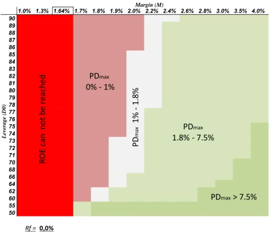
Based on risk-adjusted pricing, we first look at the one-year implied maximum PD of a project at the beginning of the construction phase. As empirics showed most project loans have a leverage above 70%, we therefore focus our simulation on the 70-90% leverage range. Table 1 shows the required minimum margin, and the maximum PDs in the construction phase according to different loan margins (M) and leverages (D0) for years 2006-2007.

(13)

13 Table 1: Implied PDmax in construction phase under conditions of 2006-2007

The minimum margin that a loan – under the given parameters – must reach is 0.79%, i.e. about 0.8%.

This is independent of leverage; and driven by the expected ROE, the general interest rate level, funding cost, and the capital adequacy ratio (see formula 4). It means, that even if the loan is expected to be risk- free (LGD is 0 and/or PD is 0), a long-term loan with a margin below 80 bps is unable to produce value to the shareholder. These cases are highlighted in red in Table 1.

Based on empirics we do not find any project types where we could assume that annual PD is greater than 1.0% (see construction projects, PPP, similar corporate ratings). Therefore, we set the next reference point at 1%. The leverage-margin pairs below the 1% implied maximum PD are presented in light red. Table 1 shows that margins less than 1.2% with a leverage higher than 75% will not produce enough expected ROE.

The next reference point can be the marginal PD of construction years of a general project. This is between 1.7%-1.9%. The less risky project of a PD between 1.0%-1.8% (highlighted in white) must have an all-in margin of 1.3-1.5% if leverage is above 75%. If we take the general average annual default rate of 7.4% of Moody’s (2013) even high leverage transactions produce enough expected ROE if the margin is above 1.5%. (Table 1 shows PDs of 1.8%-7.4% in light green, above 7.4% in dark green.) With a margin of 3% implied PD almost reaches 5% even with 90% leverage.

Kleimeier-Magginson (2005) reports project margins of the largest project launched between 1980 and 2000. Margins are spread between 56-200 bps, many of them are below 100 bps. We know from the market, business reports, interviews (Schlor 2006) that motorway PPPs in CEE launched in 2006 had

0.6% 0.7% 0.79% 0.9 1.0% 1.1% 1.2% 1.3% 1.4% 1.5% 1.6% 1.7% 1.8% 1.9% 2.0% 2.1% 3.0% 3.5% 4.0%

90 0,0% 0,0% 0,0% 0,2% 0,5% 0,7% 0,9% 1,1% 1,4% 1,6% 1,8% 2,0% 2,3% 2,5% 2,7% 3,8% 4,8% 5,9% 6,9%

89 0,0% 0,0% 0,0% 0,2% 0,5% 0,7% 0,9% 1,2% 1,4% 1,6% 1,8% 2,1% 2,3% 2,5% 2,7% 3,8% 4,9% 6,0% 7,0%

88 0,0% 0,0% 0,0% 0,2% 0,5% 0,7% 0,9% 1,2% 1,4% 1,6% 1,9% 2,1% 2,3% 2,6% 2,8% 3,9% 5,0% 6,1% 7,1%

87 0,0% 0,0% 0,0% 0,2% 0,5% 0,7% 1,0% 1,2% 1,4% 1,7% 1,9% 2,1% 2,4% 2,6% 2,8% 4,0% 5,1% 6,2% 7,2%

86 0,0% 0,0% 0,0% 0,2% 0,5% 0,7% 1,0% 1,2% 1,5% 1,7% 1,9% 2,2% 2,4% 2,7% 2,9% 4,0% 5,2% 6,3% 7,3%

85 0,0% 0,0% 0,0% 0,3% 0,5% 0,8% 1,0% 1,2% 1,5% 1,7% 2,0% 2,2% 2,5% 2,7% 2,9% 4,1% 5,3% 6,4% 7,5%

84 0,0% 0,0% 0,0% 0,3% 0,5% 0,8% 1,0% 1,3% 1,5% 1,8% 2,0% 2,3% 2,5% 2,8% 3,0% 4,2% 5,4% 6,5% 7,6%

83 0,0% 0,0% 0,0% 0,3% 0,5% 0,8% 1,0% 1,3% 1,6% 1,8% 2,1% 2,3% 2,6% 2,8% 3,1% 4,3% 5,5% 6,6% 7,8%

82 0,0% 0,0% 0,0% 0,3% 0,5% 0,8% 1,1% 1,3% 1,6% 1,8% 2,1% 2,4% 2,6% 2,9% 3,1% 4,4% 5,6% 6,8% 7,9%

81 0,0% 0,0% 0,0% 0,3% 0,5% 0,8% 1,1% 1,4% 1,6% 1,9% 2,1% 2,4% 2,7% 2,9% 3,2% 4,5% 5,7% 6,9% 8,1%

80 0,0% 0,0% 0,0% 0,3% 0,6% 0,8% 1,1% 1,4% 1,7% 1,9% 2,2% 2,5% 2,7% 3,0% 3,3% 4,6% 5,8% 7,0% 8,2%

79 0,0% 0,0% 0,0% 0,3% 0,6% 0,9% 1,1% 1,4% 1,7% 2,0% 2,3% 2,5% 2,8% 3,1% 3,3% 4,7% 6,0% 7,2% 8,4%

78 0,0% 0,0% 0,0% 0,3% 0,6% 0,9% 1,2% 1,5% 1,7% 2,0% 2,3% 2,6% 2,9% 3,1% 3,4% 4,8% 6,1% 7,4% 8,6%

77 0,0% 0,0% 0,0% 0,3% 0,6% 0,9% 1,2% 1,5% 1,8% 2,1% 2,4% 2,7% 2,9% 3,2% 3,5% 4,9% 6,3% 7,6% 8,9%

76 0,0% 0,0% 0,0% 0,3% 0,6% 0,9% 1,2% 1,5% 1,8% 2,1% 2,4% 2,7% 3,0% 3,3% 3,6% 5,0% 6,4% 7,8% 9,1%

75 0,0% 0,0% 0,0% 0,3% 0,6% 1,0% 1,3% 1,6% 1,9% 2,2% 2,5% 2,8% 3,1% 3,4% 3,7% 5,2% 6,6% 8,0% 9,4%

74 0,0% 0,0% 0,0% 0,3% 0,7% 1,0% 1,3% 1,6% 2,0% 2,3% 2,6% 2,9% 3,2% 3,5% 3,8% 5,4% 6,8% 8,2% 9,6%

73 0,0% 0,0% 0,0% 0,3% 0,7% 1,0% 1,4% 1,7% 2,0% 2,4% 2,7% 3,0% 3,3% 3,7% 4,0% 5,5% 7,0% 8,5% 9,9%

72 0,0% 0,0% 0,0% 0,4% 0,7% 1,1% 1,4% 1,8% 2,1% 2,4% 2,8% 3,1% 3,5% 3,8% 4,1% 5,7% 7,3% 8,8% 10,3%

71 0,0% 0,0% 0,0% 0,4% 0,7% 1,1% 1,5% 1,8% 2,2% 2,5% 2,9% 3,2% 3,6% 3,9% 4,3% 5,9% 7,6% 9,1% 10,6%

70 0,0% 0,0% 0,0% 0,4% 0,8% 1,2% 1,5% 1,9% 2,3% 2,6% 3,0% 3,4% 3,7% 4,1% 4,4% 6,2% 7,9% 9,5% 11,0%

68 0,0% 0,0% 0,0% 0,4% 0,8% 1,3% 1,7% 2,1% 2,5% 2,9% 3,3% 3,7% 4,1% 4,5% 4,9% 6,8% 8,6% 10,3% 12,0%

66 0,0% 0,0% 0,0% 0,5% 0,9% 1,4% 1,9% 2,3% 2,8% 3,2% 3,7% 4,1% 4,5% 5,0% 5,4% 7,5% 9,5% 11,4% 13,2%

64 0,0% 0,0% 0,0% 0,5% 1,1% 1,6% 2,1% 2,6% 3,2% 3,7% 4,2% 4,7% 5,2% 5,6% 6,1% 8,5% 10,7% 12,8% 14,8%

62 0,0% 0,0% 0,0% 0,6% 1,3% 1,9% 2,5% 3,1% 3,7% 4,3% 4,9% 5,4% 6,0% 6,6% 7,1% 9,8% 12,3% 14,7% 17,0%

60 0,0% 0,0% 0,0% 0,8% 1,6% 2,3% 3,1% 3,8% 4,5% 5,2% 5,9% 6,6% 7,3% 8,0% 8,6% 11,8% 14,8% 17,5% 20,1%

55 0,0% 0,0% 0,0% 2,2% 4,4% 6,4% 8,4% 10,3% 12,1% 13,9% 15,5% 17,1% 18,7% 20,2% 21,6% 28,1% 33,6% 38,3% 42,4%

50 0,0% 0,0% 0,0% 11,2% 20,2% 27,5% 33,6% 38,7% 43,1% 46,9% 50,3% 53,2% 55,8% 58,1% 60,2% 68,2% 73,5% 77,3% 80,2%

Margin (M)

Leverage (D0) ROE can not be reached

PD^max 0% - 1%

PD^max 1% - 1.8%

PD^max> 7.5%

PD^max 1.8% - 7.5%

Rf = 3,5%

CV = 55%

c = 6%

L = 0,3%

ROE = 12%

(14)

14 (have) a margin of about 1.2% with a leverage of close to 90%. By 2007-2008 these margins – when banking consortiums were formed at the start of the project – went down further to 1% and leverages went up to 90%. There are market comments stating that margins went down even to 0.6-0.7% (Bain 2009, pp 29). We can conclude that even with an average recovery outlook projects under 1.2% all-in margins were very unlikely to be priced properly. Moreover, those loans where pricing fell below 1%

(as in PPPs of 2007-2008) certainly did not produce a value added to shareholders. Easing the leverage to 65-75% – which often happened in the period of crisis – could largely improve the opportunity to produce the required ROE even with smaller margins.

We repeat our simulation in the case of the operation phase. In this case recovery, default statistics, and all reference points improve. Average recoveries are about 80%, so we set collateral value (CV) at 75%, which harmonizes with these empirics. This means that with a leverage of equal or better than 75% the expected LGD and therefore EL is 0.

Table 2: Implied PDmax in operation phase under conditions of 2006-2007

We know that marginal PDs of an average project fall after three years and go below 1% after the fifth year. However, the minimum margin is independent of risk and recovery. Below a margin of 0.79%, there is no value added loan under these parameters. But in the operation phase, a loan at high leverage (85-90%), with a margin of 1.0%-1.1% could produce enough expected ROE. With these recoveries, a relatively low leverage of 70% and a margin of 1%-1.1% is surely enough for creating value for shareholders. Equity sponsors and banks were aware of the decrease in risk level after the construction

0,6% 0.7% 0.79% 0.8% 1.0% 1.1% 1.2% 1.3% 1.4% 1.5% 1.6% 1.7% 1.8% 1.9% 2.0% 2.5% 3.0% 3.5% 4.0%

90 0,0% 0,0% 0,0% 0,5% 1,0% 1,4% 1,9% 2,4% 2,8% 3,3% 3,7% 4,1% 4,6% 5,0% 5,4% 7,5% 9,5% 11,4% 13,2%

89 0,0% 0,0% 0,0% 0,5% 1,0% 1,5% 2,0% 2,5% 2,9% 3,4% 3,9% 4,3% 4,8% 5,2% 5,7% 7,8% 9,9% 11,9% 13,8%

88 0,0% 0,0% 0,0% 0,6% 1,1% 1,6% 2,1% 2,6% 3,1% 3,6% 4,1% 4,5% 5,0% 5,5% 5,9% 8,2% 10,3% 12,4% 14,4%

87 0,0% 0,0% 0,0% 0,6% 1,1% 1,7% 2,2% 2,7% 3,2% 3,8% 4,3% 4,8% 5,3% 5,8% 6,2% 8,6% 10,8% 13,0% 15,0%

86 0,0% 0,0% 0,0% 0,6% 1,2% 1,8% 2,3% 2,9% 3,4% 4,0% 4,5% 5,0% 5,6% 6,1% 6,6% 9,1% 11,4% 13,6% 15,8%

85 0,0% 0,0% 0,0% 0,7% 1,3% 1,9% 2,5% 3,1% 3,6% 4,2% 4,8% 5,3% 5,9% 6,4% 7,0% 9,6% 12,0% 14,4% 16,6%

84 0,0% 0,0% 0,0% 0,7% 1,4% 2,0% 2,6% 3,3% 3,9% 4,5% 5,1% 5,7% 6,3% 6,8% 7,4% 10,2% 12,8% 15,2% 17,6%

83 0,0% 0,0% 0,0% 0,8% 1,5% 2,2% 2,8% 3,5% 4,2% 4,8% 5,5% 6,1% 6,7% 7,3% 7,9% 10,9% 13,6% 16,2% 18,7%

82 0,0% 0,0% 0,0% 0,8% 1,6% 2,3% 3,1% 3,8% 4,5% 5,2% 5,9% 6,6% 7,3% 7,9% 8,6% 11,7% 14,6% 17,4% 19,9%

81 0,0% 0,0% 0,0% 0,9% 1,7% 2,6% 3,4% 4,1% 4,9% 5,7% 6,4% 7,2% 7,9% 8,6% 9,3% 12,7% 15,8% 18,7% 21,4%

80 0,0% 0,0% 0,0% 1,0% 1,9% 2,8% 3,7% 4,6% 5,4% 6,3% 7,1% 7,9% 8,7% 9,5% 10,2% 13,9% 17,2% 20,3% 23,2%

79 0,0% 0,0% 0,0% 1,1% 2,2% 3,2% 4,2% 5,1% 6,1% 7,0% 7,9% 8,8% 9,7% 10,5% 11,4% 15,4% 19,0% 22,3% 25,4%

78 0,0% 0,0% 0,0% 1,3% 2,5% 3,6% 4,7% 5,8% 6,9% 7,9% 9,0% 10,0% 10,9% 11,9% 12,8% 17,2% 21,2% 24,8% 28,1%

77 0,0% 0,0% 0,0% 1,5% 2,9% 4,2% 5,5% 6,8% 8,0% 9,2% 10,4% 11,6% 12,7% 13,7% 14,8% 19,7% 24,1% 28,0% 31,6%

76 0,0% 0,0% 0,0% 1,9% 3,5% 5,2% 6,7% 8,2% 9,7% 11,1% 12,5% 13,8% 15,1% 16,3% 17,6% 23,2% 28,0% 32,3% 36,1%

75 0,0% 0,0% 0,0% 2,4% 4,6% 6,6% 8,6% 10,4% 12,3% 14,0% 15,7% 17,3% 18,8% 20,3% 21,7% 28,2% 33,6% 38,3% 42,4%

74 0,0% 0,0% 0,0% 3,5% 6,5% 9,3% 12,0% 14,5% 16,8% 19,1% 21,2% 23,2% 25,1% 27,0% 28,7% 36,3% 42,4% 47,4% 51,7%

73 0,0% 0,0% 0,0% 6,3% 11,4% 16,0% 20,2% 23,9% 27,4% 30,5% 33,4% 36,0% 38,4% 40,7% 42,8% 51,4% 57,8% 62,7% 66,5%

72 0,0% 0,0% 0,0% 12,0% 20,8% 28,0% 34,0% 39,1% 43,4% 47,2% 50,5% 53,4% 56,0% 58,3% 60,4% 68,3% 73,6% 77,4% 80,2%

71 0,0% 0,0% 0,0% 12,0% 20,8% 28,0% 34,0% 39,1% 43,4% 47,2% 50,5% 53,4% 56,0% 58,3% 60,4% 68,3% 73,6% 77,4% 80,2%

70 0,0% 0,0% 0,0% 12,0% 20,8% 28,0% 34,0% 39,1% 43,4% 47,2% 50,5% 53,4% 56,0% 58,3% 60,4% 68,3% 73,6% 77,4% 80,2%

68 0,0% 0,0% 0,0% 12,0% 20,8% 28,0% 34,0% 39,1% 43,4% 47,2% 50,5% 53,4% 56,0% 58,3% 60,4% 68,3% 73,6% 77,4% 80,2%

66 0,0% 0,0% 0,0% 12,0% 20,8% 28,0% 34,0% 39,1% 43,4% 47,2% 50,5% 53,4% 56,0% 58,3% 60,4% 68,3% 73,6% 77,4% 80,2%

64 0,0% 0,0% 0,0% 12,0% 20,8% 28,0% 34,0% 39,1% 43,4% 47,2% 50,5% 53,4% 56,0% 58,3% 60,4% 68,3% 73,6% 77,4% 80,2%

62 0,0% 0,0% 0,0% 12,0% 20,8% 28,0% 34,0% 39,1% 43,4% 47,2% 50,5% 53,4% 56,0% 58,3% 60,4% 68,3% 73,6% 77,4% 80,2%

60 0,0% 0,0% 0,0% 12,0% 20,8% 28,0% 34,0% 39,1% 43,4% 47,2% 50,5% 53,4% 56,0% 58,3% 60,4% 68,3% 73,6% 77,4% 80,2%

55 0,0% 0,0% 0,0% 12,0% 20,8% 28,0% 34,0% 39,1% 43,4% 47,2% 50,5% 53,4% 56,0% 58,3% 60,4% 68,3% 73,6% 77,4% 80,2%

50 0,0% 0,0% 0,0% 12,0% 20,8% 28,0% 34,0% 39,1% 43,4% 47,2% 50,5% 53,4% 56,0% 58,3% 60,4% 68,3% 73,6% 77,4% 80,2%

ROE can not be reached PDmax 0% -1% PDmax 1% -1.8%