Interest premium and external position: a time varying approach

MŰHELYTANULMÁNYOK DISCUSSION PAPERS

MT-DP – 2018/29

Interest premium and external position:

a time varying approach

ISTVÁN KÓNYA – FRANKLIN MADUKO

Discussion papers MT-DP – 2018/29

Institute of Economics, Centre for Economic and Regional Studies, Hungarian Academy of Sciences

KTI/IE Discussion Papers are circulated to promote discussion and provoque comments.

Any references to discussion papers should clearly state that the paper is preliminary.

Materials published in this series may subject to further publication.

Interest premium and external position: a time varying approach

Authors:

István Kónya senior research fellow

Center of Economics and Regional Sciences – Institute of Economics Hungarian Academy of Sciences

University of Pécs, and Central European University email: konya.istvan@krtk.mta.hu

Franklin Maduko graduate student

Central European University, Economics Department

November 2018

Interest premium and external position:

a time varying approach

István Kónya - Franklin Maduko

Abstract

The paper reexamines the empirical relationship between external indebtedness and the interest premium on government bonds. We use a broad sample of countries between 1980- 2017 that includes advanced, emerging and less-developed economies. We show that the relationship is strongly state-dependent, and it varies both with the international financial climate, and with the level of development. Moreover, while we find some evidence for non- linearity, this is mostly driven by turbulent periods. We carry out a number of robustness exercises, which highlight issues related to sample composition, the choice of the debt measure, and the definition of crisis events.

JEL: F34, F41, E43, E44

Keywords: interest premium, net foreign assets, estimation, country panel, state dependence

Acknowledgement:

This research was supported by: (1) the Higher Education Institutional Excellence Program of the Ministry of Human Capacities in the framework of the 'Financial and Public Services' research project (1783-3/2018/FEKUTSTRAT) at Corvinus University of Budapest, and (2) by The National Research, Development and Innovation Office of Hungary (OTKA K116033).

Konya also received the Bolyai Scholarship of the Hungarian Academy of Sciences during while working on the topic. He would like to thank the National Bank of Poland for their hospitality and professional support.

Kamatprémium és külső pozíció:

egy időben változó megközelítés

Kónya István - Franklin Maduko

Összefoglaló

A tanulmány a külső eladósodottság és a kormányzati kötvényekre fizetett kamatprémium közötti empirikus kapcsolatot vizsgálja. Ehhez egy széles országmintát használunk 1980–

2017 között, amelyben találhatók fejlett, felzárkózó és fejlődő gazdaságok is. Megmutatjuk, hogy a kapcsolat erősen állapotfüggő, és változik a nemzetközi pénzügyi hangulat, valamint a gazdasági fejlettség függvényében. Emellett megfigyelhető nemlinearitás is, de ez elsősorban az instabil időszakokra jellemző. Számos robusztusság vizsgálatot is elvégzünk, amelyek a minta összetételére, az eladósodottság mérőszámának megválasztására, valamint a krízisepizódok definiálására vonatkoznak.

Tárgyszavak: kamatprémium, nettó külső pozíció, becslés, országpanel, állapotfüggőség

JEL: F34, F41, E43, E44

Interest premium and external position: a time varying approach ^∗

Istvan Konya

Franklin Maduko

November 5, 2018

Abstract

The paper reexamines the empirical relationship between external indebt- edness and the interest premium on government bonds. We use a broad sample of countries between 1980-2017 that includes advanced, emerging and less-developed economies. We show that the relationship is strongly state- dependent, and it varies both with the international financial climate, and with the level of development. Moreover, while we find some evidence for non- linearity, this is mostly driven by turbulent periods. We carry out a number of robustness exercises, which highlight issues related to sample composition, the choice of the debt measure, and the definition of crisis events.

JEL codes: F34, F41, E43, E44

∗This research was supported by: (1) the Higher Education Institutional Excellence Program of the Ministry of Human Capacities in the framework of the ’Financial and Public Services’

research project (1783-3/2018/FEKUTSTRAT) at Corvinus University of Budapest, and (2) by The National Research, Development and Innovation Office of Hungary (OTKA K116033). Konya also received the Bolyai Scholarship of the Hungarian Academy of Sciences during while working on the topic. He would like to thank the National Bank of Poland for their hospitality and professional support.

†Center for Economic and Regional Studies (Hungarian Academy of Sciences), University of P´ecs, and Central European University

‡Central European University

Keywords: interest premium, net foreign assets, estimation, country panel, state dependence

1 Introduction

The effect of indebtedness on the external interest premium has been of great the- oretical and empirical interest in international macroeconomics. On the empirical side, the conditions under which countries can borrow from abroad differ greatly.

An obvious explanation is that markets assign different probabilities to default, ei- ther sovereign or private. If default risk is positively correlated with the extent of indebtedness, this creates a link between the level of debt and the external premium.

On the theoretical side, debt-dependent interest premia are introduced into open economy macro models to induce stationarity on the one hand, and as a simple stand- in for financial frictions on international capital markets on the other hand. Since Schmitt-Groh´e and Uribe (2003), a positive debt elasticity of the external interest rate is a regular feature of small open economy models.

The exact relationship between measures of indebtedness and external interest rates, however, remains elusive. Macroeconomic models where a debt-dependent interest rate was introduced to guarantee stationarity, starting with Schmitt-Groh´e and Uribe (2003), tended to use a small value for the elasticity parameter. Estimated DSGE models tended to find larger values, such as Garc´ıa-Cicco, Pancrazzi and Uribe (2010). In these latter models the debt dependent interest rate stands in for financial frictions, which helps explain the dynamics of consumption and the trade balance.

Another strand of the literature tried to uncover whether the relationship be- tween the external interest premium and indebtedness is nonlinear. In a model of the global financial crisis of 2009-2010, Bencz´ur and K´onya (2016) assume a Linex specification, and show that this is important to match quantitatively the differ-

ent experience of four Central-Eastern European economies (the Czech Republic, Hungary, Poland and Slovakia) during the 2008-2009 financial crisis. A recent con- tribution to the empirical literature on potential non-linearity is Brzoza-Brzezina and Kotlowski (2016). The paper estimates a regime switching regression, where the regimes are linked to the extent of external indebtedness. Findings indicate that the interest premium - debt relationship is indeed non-linear in their sample, and non-linearity becomes important when the net foreign asset (NFA) - GDP ratio reaches about -70-75%.

In this paper we revisit the empirical findings and qualify them in a number of ways. Our main question is the following: is the debt-premium relationship state-dependent? The topic is partly motivated by discussions of a global financial cycle (Rey, 2013; Passari and Rey, 2015), which posits that financing conditions of individual countries vary with the global appetite for risk. It is reasonable to expect that the debt-premium relationship varies with global - or possibly regional or even local - conditions. The already mentioned work of Bencz´ur and K´onya (2016) model the financial crisis as a permanent shift in the premium function. The debt-premium relationship may also depend on the level of economic development. In general, the level of sustainable debt relative to GDP is considered lower in emerging countries than in advanced economies. This may be a result of lower trust in the economic policies followed by the former group. Therefore, we also test for state dependence with respect to relative GDP per capita.

Our findings indicate that the debt-premium relationship is indeed state depen- dent. The relationship is much stronger during crisis times, and its strength also decreases with the level of economic development. We find some evidence of non- linearity, but primarily during crisis times. In terms of macroeconomic modeling, our results are consistent with regime switching frameworks (see for example Blagov, 2018), where tranquil and turbulent periods alternate and are accompanied by dif- ferent debt-premium functional relationships. After presenting the baseline results

we run a number of robustness checks where we vary the sample, the measure of debt, and the definition of crisis events.

Besides Brzoza-Brzezina and Kotlowski (2016), our work is most closely related to Dell’Erba, Hausmann and Panizza (2013). These authors estimate the relation- ship between sovereign spreads and government debt. Similarly to our work, they look at differences across emerging and advanced economies, and across turbulent and tranquil times. In addition, they study whether the currency composition of external debt matters for the spreads. In general, they find state dependence similar to our results.

Our work extends and compliments Brzoza-Brzezina and Kotlowski (2016, BK henceforth) and Dell’Erba, Hausmann and Panizza (2013, DHP henceforth) in a number of ways. First, we use a much broader sample than either of these papers.

We mostly add less developed countries and a longer time period - our sample starts in 1980 and ends in 2017. Second, we combine the approaches in the two papers, and look both for state dependence and non-linearity. Third, in contrast to DHP, we use interest rates on long government bonds to measure sovereign spreads instead of EMBI spreads (their measure for emerging economies). This allows us to work with a much longer sample period. Also, over time the EMBI measure became less relevant for emerging countries, because they are increasingly able to borrow in their own currencies, and the EMBI only tracks dollar-denominated bonds.

This casts some doubt on results that use this index as a measure of the relevant spread.¹ The disadvantage of using bond yields, on the other hand, is that we cannot control for the currency of issuance - we return to this issue later. Forth, we add number of additional specifications. We look at a much broader set of crisis events, compare different measures of indebtedness (the net foreign asset position and gross government debt), and discuss potential sample selection problems.

Our paper is also related to the work on the determinants of emerging econ-

1https://www.economist.com/finance-and-economics/2007/02/22/bye-bye-embi

omy bond spreads. A˘gca and Celasun (2012) use firm-loan level data to estimate determinants on yield spread for the private sector. They find that there are sig- nificant spillovers from external public debt and private spreads, but they find no relationship between domestic public debt and spreads. This supports our use of the overall net foreign asset position as the main measure of aggregate indebted- ness. Similarly to DHP, Comelli (2012) also uses the EMBI spread as a measure of the interest premium, and focuses on emerging markets. He also finds that the debt-premium relationship depends on global economic conditions. In contrast to our paper, however, he does not include measures of indebtedness as an explanatory variable. Csont´o (2014) studies the interactions between global financial conditions and country-level fundamentals, also focusing on emerging economies.

The paper is organized as follows. First, we discuss our sample and some mea- surement issues in Section 2. Next we turn to our baseline results, including tests of state dependence and non-linearity in Section 3. Then we present a number of robustness exercises in Section 4. Finally, Section 5 concludes.

2 Measurement

Our full sample consists of an annual unbalanced panel data for 89 advanced, emerg- ing and developing countries between 1980-2017. The unbalanced nature results from limited availability of long term interest rate data for many countries in some - typically the earlier - time periods. Only some advanced countries have continuous interest rate coverage for most of the years. Others enter the sample later, and some countries also experience gaps.

We make two additional adjustments to the sample we use for estimation. First, we drop very small countries (with population on average below 1 million), based on the assumption that their behavior is highly idiosyncratic. These countries are Botswana, Cyprus, Fiji, Iceland, Luxembourg, Maldives, Malta, Mauritius, Samoa,

Seychelles, Solomon Islands and Vanuatu. Second, we remove country-year obser- vations where inflation is persistently high. We define such high inflation episodes as ones where the five-year average inflation rate is above 10%, starting from the year in question. The rational is that calculating the real interest rate is highly unreliable in these cases, and when inflation is very high, ex-post real interest rates - and hence interest premia - can easily be significantly negative, but it is unlikely that this is due to favorable treatment by financial markets. We experimented with other thresholds, and results are robust to the precise definition.

Our final, restricted sample is presented in Table 1. We believe that this sample is appropriate for our analysis, as it includes a broad set of countries and time periods that can be considered “normal” or “representative”. Note that even after we drop small countries and high inflation observations, we still have many more countries and periods than Brzoza-Brzezina and Kotlowski (2016) or Dell’Erba, Hausmann and Panizza (2013). Our main results will be derived from this sample, but we include robustness check for the original, full sample in a later section.

The two key variables that we need for the estimation are a measure of the interest premium and a measure of external indebtedness. We follow Brzoza-Brzezina and Kotlowski (2016) and use the net foreign asset position (NFA) over GDP ratio as our main measure of debt, although later we report robustness results with the gross debt position of the general government as in Dell’Erba, Hausmann and Panizza (2013). For the interest rate, we use long government bond rates. The premium is constructed as a difference of these rates and the long bond yield for the United States. Ideally one would need bond yields in the same currency, preferably in US dollars. Unfortunately data availability is very limited for such instruments. Also, as we discussed earlier, dollar spread measures such as the EMBI are becoming less representative of overall market sentiment. Therefore, we again follow BK and include the inflation differential between a country and the United States as a right- hand side variable to control for expected exchange rate movements. Our inflation

Table 1: List of Countries

Country Period Country Sample

Armenia 2000-2017 Malaysia 1992-2017

Australia 1980-2017 Mali 2014

Austria 1980-2017 Mexico 2000-2017

Bangladesh 2006-2017 Moldova 2005-2017

Belgium 1980-2017 Mongolia 2013-2017

Benin 2015 Morocco 1997-2007, 2010-2017

Brazil 2007, 2010-2017 Myanmar 2010-2017

Bulgaria 2003-2017 Namibia 1994-2010, 2012

Burkina Faso 2012-2015 Nepal 1981, 1987, 1993-2017

Canada 1980-2017 Netherlands 1981, 1987-2017

Chile 2005-2017 New Zealand 1986-2017

China 2005-2017 Niger 2014-2015

Colombia 2003-2017 Norway 1985-2017

Costa Rica 2014-2016 Pakistan 1992, 1995-1998

2001-2004, 2011-2017

Cote d’Ivoire 2012-2013 Papua New Guinea 2005-2017

Czech Republic 2000-2017 Philippines 1994-2007, 2014

Denmark 1980-2017 Poland 2001-2017

Estonia 1997-2010 Portugal 1990-2017

Ethiopia 1986-1987, 1992-1997 Romania 2005-2017

Finland 1987-2017 Russia 2008-2017

France 1981-2017 Senegal 2012-2015

Germany 1980-2017 Singapore 1999-2017

Ghana 2009-2010 Slovakia 2000-2017

Greece 1993-2017 Slovenia 2002-2017

Honduras 1983-1986, 1999-2007 South Africa 1992-2017

Hungary 2000-2017 Spain 1983-2017

India 1981-1985, 1993-2017 Sri Lanka 2009-2017

Indonesia 2003-2017 Sweden 1981-2017

Ireland 1982-2017 Switzerland 1980-2017

Israel 1997-2017 Thailand 1999-2017

Italy 1983-2017 Togo 2012-2015

Jamaica 1997-1998 Trinidad and Tobago 1984-1993

Japan 1989-2017 Turkey 2010-2016

Korea 1981-2017 Uganda 2009

Kyrgyzstan 2009-2017 United Kingdom 1980-2017

Latvia 2001-2017 United States 1980-2017

Lithuania 2001-2017 Uruguay 2011-2017

measure for year t is 5-year moving average between t and t+4. We use actual observations when available. For years 2014-2017, when averaging takes us past the sample period, we rely on inflation forecasts in the IMF World Economic Outlook.

We use the following set of independent variables, including the two just de- scribed and additional controls.

1. Net Foreign Assets to GDP ratio.

• Data comes from two sources. The principal source is the updated dataset described in Lane and Milesi-Feretti (2018, LMF henceforth), which con- tains data until 2015. We add observations for 2016 and 2017 using the IMF Balance of Payments statistics.

2. Long-term interest rate on government bonds.

• The principal data source is the IMF International Financial Statistics. In a few cases, we augment this with observations from the OECD Statistics, and Bloomberg.

3. General government gross debt to GDP ratio, current account, GDP (both real, nominal and purchasing power parity), budget balance, inflation.

• The data source for these variables is the World Economic Outlook.

4. Foreign exchange reserves to GDP ratio.

• The main source is the LMF database, augmented with IFS for 2016-2017.

5. Exchange rate volatility.

(a) Data comes from the Bank for International Settlements and Interna- tional Financial Statistics.

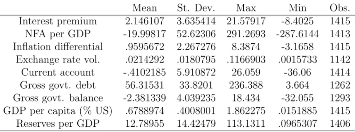
Table 2 presents descriptive statistics for the main variables.

Mean St. Dev. Max Min Obs.

Interest premium 2.146107 3.635414 21.57917 -8.4025 1415 NFA per GDP -19.99817 52.62306 291.2693 -287.6144 1413 Inflation differential .9595672 2.267276 8.3874 -3.1658 1415 Exchange rate vol. .0214292 .0180795 .1166903 .0015733 1142 Current account -.4102185 5.910872 26.059 -36.06 1414 Gross govt. debt 56.31531 33.8201 236.388 3.664 1262 Gross govt. balance -2.381339 4.039235 18.434 -32.055 1293 GDP per capita (% US) .6788974 .4008001 1.862275 .0151885 1415 Reserves per GDP 12.78955 14.42479 113.1311 .0965307 1406

Table 2: Descriptive statistics

3 Empirical results

The regressions we run take the generic form given in equation (1):

y_it =α+β₁N F A_it+γ⁰x_it+µ_i+η_t+_it, (1)

where yit is the long-term interest rate premium of country i in time t, NFA is the net foreign asset to GDP ratio, x_it is a vector of various covariates, µ_i is a country fixed effect, andη_tis a year fixed effect. This regression is similar to the preliminary specification in BK, with the additional countries included in the sample and time dummies added. Time dummies are important, since global financial conditions vary over time, and this is likely to be reflected in country specific risk premia.

Our main goal is to investigate various sources of state dependence. Our main questions are the following.

1. Is the NFA - premium relationship present in our sample, and if yes what is the magnitude of the estimated parameter?

2. Does the presence of time dummies significantly change the result?

3. Is the debt-premium slope parameter time dependent? In particular, does it increase in times of financial turbulance (i.e. crisis)?

countries?

In our baseline specification, we use a very simple definition of crisis episodes. We simply assume that global financial markets were turbulent during the “long” global financial crisis of 2008-2013, which includes the subsequent Euro crisis as well. This is motivated to a large extent by data limitations: our coverage of emerging economies is very patchy until 2000, whereas earlier crisis tended to concentrate among them.

Also, the global financial crisis affected all countries to varying degrees, while earlier events - such as the East Asian crisis starting in 1997 - were geographically more limited. In a robustness exercise later, we present results with alternative crisis definitions as well.

3.1 Baseline results

We estimate equation (1) with various controls included. The baseline results are reported in Table 3, and our additional findings are reported in Table 4. The tables are split so that we first present results comparable to earlier findings, and then we turn to testing state dependence in the debt-premium relationship.

The first column in Table 3 is the simple linear specification, where the nominal interest premium is regressed on the lagged NFA-GDP ratio with only the 5-year inflation differential relative to the US as a control variable. We also include country fixed effects in all the specification. The second column adds additional controls:

GDP per capita relative to the US, the volatility of the nominal exchange rate, the current account, central bank reserves and the budget balance as percentages of GDP. The third column includes year dummies, to control for general changes in the global appetite for risk.

The results show that the level of indebtedness has a significant, but fairly modest impact on the interest rate premium. A 10 percentage point deterioration in the NFA-GDP ratio leads to a 8.36-11.6 basis point increase in the interest premium,

Table 3: Baseline results

(1) (2) (3)

Lagged NFA/GDP -0.0116*** -0.00984*** -0.00836***

[0.00252] [0.00261] [0.00241]

Infl. diff. 0.341*** 0.345*** 0.310***

[0.0486] [0.0601] [0.0619]

Relative GDP -3.354*** -5.734***

[1.262] [1.210]

NEER volatility 19.33*** 15.92***

[4.173] [4.127]

Current acc. 0.0334** 0.0542***

[0.0157] [0.0145]

Reserves 0.00874 0.00197

[0.00872] [0.00807]

Budget bal. -0.173*** -0.0795***

[0.0193] [0.0207]

NFA x Crisis NFA squared

NFA squared x Crisis NFA x Rel. GDP

NFA x Crisis x Rel. GDP

Constant 1.529*** 2.506*** 4.424***

[0.0940] [0.858] [1.090]

Country FE yes yes yes

Year FE no no yes

Observations 1,352 1,013 1,013

R squared 0.043 0.145 0.333

Standard errors in parentheses

* p<0.10, ** p<0.05, *** p<0.01

used in Schmitt-Groh´e and Uribe (2003), but in line with estimated DSGE models such as Jakab and K´onya (2015) and also very similar to the coefficient in BK. The coefficients on the other controls are mostly as expected, although the positive sign on the current account might indicate reverse causality, if troubled countries are switching to current account surpluses to improve their balance sheets.

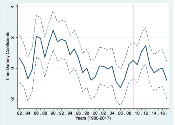
Time dummies are important, and change the estimated coefficient significantly (it drops by about one-third). The explanatory power of the regression doubles relative to the regression with the same controls, but without time dummies. Figure 1 plots the year dummy coefficients, which are also instructive on their own right. We can see that global financial conditions - captured by the interest premium relative to the US - do vary over time. Most importantly, the estimation identifies the general decline in premia over the 1990s and 2000s until the financial crisis. As expected, the global premium component starts rising from 2007, and peaks in 2012. This latter finding might be driven by the fact that we have many European countries in the sample, and there was a secondary crisis in the Euro area between 2011-2013.

Figure 1: Time dummies in the baseline specification

Table 4 turns to the question of state dependence in the debt-premium relation- ship. We look for two such possibilities. In the first column we add an interaction term between the NFA - GDP ratio and the crisis dummy, defined to be 1 during the broadly interpreted global financial crisis of 2008-2013. We later report robustness check with different crisis definitions.

Controlling for the financial crisis is important. While still significant, the coef- ficient is now lower in tranquil times. The coefficient in crisis times, on the other hand, is almost twice as high as the average estimated earlier (column [3] above).

That the crisis interaction is highly significant and quantitatively dominant implies that the debt-premium relationship is mostly driven by turbulent periods.

The second column tests for non-linearity. On its own, the quadratic term is not significant. While this is a cruder approach than the regime-switching regression in BK, our findings indicate that non-linearity is not a general feature. In fact, even the linear term becomes almost insignificant during normal times. When we interact the quadratic term with the crisis dummy, however, we get a significant coefficient, along with the crisis dummy itself. For a country that has no debt (NFA/GDP = 0), the marginal effect is−0.004 in normal times, and equals−0.017 in crisis times. For a country with an NFA/GDP position equal to -50%, the marginal effect is the same in normal times, but becomes−0.22 in crisis times. This means that a further 10%

decline in the NFA-GDP ratio would lead to a 2 percentage point increase in the interest premium. This may be unreasonably high and could be further refined by a more sophisticated definition of non-linearity. Nevertheless, the general message is that potentially strong non-linearity appears only in turbulent periods.

The second form of state dependence we test for considers relative development.

We ask whether countries with lower GDP per capita relative to the United States face a steeper debt-premium relationship. Column (6) in Table 4 shows that this is indeed the case. First, the interaction term is highly significant and quantitatively large. For a country with the same GDP per capita as the US, the interest premium

Table 4: State dependence

(4) (5) (6)

Lagged NFA/GDP -0.00662*** -0.00436* -0.0204***

[0.00244] [0.00249] [0.00591]

Infl. diff. 0.344*** 0.364*** 0.384***

[0.0621] [0.0618] [0.0621]

Relative GDP -5.171*** -5.486*** -5.268***

[1.212] [1.203] [1.208]

NEER volatility 15.51*** 13.99*** 14.74***

[4.100] [4.076] [4.068]

Current acc. 0.0585*** 0.0608*** 0.0635***

[0.0145] [0.0145] [0.0144]

Reserves 0.00473 0.00236 0.00731

[0.00805] [0.00800] [0.00819]

Budget bal. -0.0715*** -0.0723*** -0.0837***

[0.0207] [0.0205] [0.0207]

NFA x Crisis -0.00824*** -0.0113*** -0.0213***

[0.00224] [0.00235] [0.00540]

NFA squared 9.45e-06

[1.35e-05]

NFA squared x Crisis 8.11e-05***

[1.90e-05]

NFA x Rel. GDP 0.0139***

[0.00506]

NFA x Crisis x Rel. GDP 0.0129***

[0.00464]

Constant 3.982*** 4.179*** 3.644***

[1.090] [1.081] [1.095]

Country FE yes yes yes

Year FE yes yes yes

Observations 1,013 1,013 1,013

R squared 0.337 0.35 0.352

Standard errors in parentheses

* p<0.10, ** p<0.05, *** p<0.01

is−0.0204+1×0.0139 =−0.0065. For a country whose GDP per capita is 50% of the US level, the premium is−0.0204 + 0.5×0.0145 =−0.0135. Relative development matters even more in crisis periods. In turbulent times, the coefficient on NFA/GDP is (−0.0204−0.0213) + 1×(0.0139 + 0.0129) = −0.0149 for the hypothetical rich country, and (−0.0204−0.0213) + 0.5×(0.0139 + 0.0129) =−0.283 for the poorer economy.

These results are consistent with a “safe haven” interpretation. During times of international financial problems, investors tend to seek safe assets, such as US treasuries, German bunds and other rich country bonds. As the appetite for risk declines, financial markets are particularly weary to invest into less developed, highly indebted economies. This drives up the interest premium for such countries more than for rich economies. A caveat to these results is that our crisis identification primarily comes from the global financial crisis, when these issues were particularly prevalent. We return to this issue in the next section.

4 Robustness

4.1 Full sample

Table 5 presents results for the full sample, where we include both small countries and high inflation episodes. The four columns include the baseline specifications with controls, and the tests of state dependence and non-linearity that we discussed in the previous section for the preferred sample. In general the results are much weaker, and the coefficients are often insignificant. The NFA/GDP coefficient is about one-third of what we found in the restricted sample. The crisis dummy and the crisis interaction are small and insignificant, although they have the expected sign. Relative GDP and its interaction with indebtedness are still significant, and the estimated coefficients are similar to the previous results.

An indication that this sample is not suitable for analysis is the extremely small

Table 5: State dependence

(7) (8) (9) (10)

Lagged NFA/GDP -0.00380** -0.00366* -0.00528** -0.0159***

[0.00155] [0.00202] [0.00233] [0.00483]

Infl. diff. -0.000521** -0.000522** -0.000508** -0.000485**

[0.000227] [0.000227] [0.000227] [0.000228]

Relative GDP -7.591*** -7.575*** -7.443*** -7.492***

[1.371] [1.380] [1.382] [1.380]

NEER volatility 27.58*** 27.57*** 27.81*** 27.39***

[3.509] [3.514] [3.515] [3.502]

Current acc. 0.0380*** 0.0381*** 0.0392*** 0.0374***

[0.0143] [0.0143] [0.0144] [0.0144]

Reserves -0.0169** -0.0170** -0.0133 -0.0139*

[0.00799] [0.00803] [0.00830] [0.00820]

Budget bal. -0.0298 -0.0296 -0.0279 -0.0378*

[0.0210] [0.0210] [0.0210] [0.0212]

NFA x Crisis -0.000220 -0.00261 -0.00432

[0.00200] [0.00241] [0.00578]

NFA squared -1.06e-06

[8.55e-06]

NFA squared x Crisis -8.59e-06

[8.38e-06]

NFA x Rel. GDP 0.0116***

[0.00402]

NFA x Crisis x Rel. GDP 0.00523

[0.00523]

Constant 6.986*** 6.980*** 6.830*** 6.669***

[1.188] [1.191] [1.193] [1.194]

Country FE yes yes yes yes

Year FE yes yes yes yes

Observations 1,204 1,204 1,204 1,204

R squared 0.276 0.276 0.278 0.283

Standard errors in parentheses

* p<0.10, ** p<0.05, *** p<0.01

- but significantly negative - coefficient on the inflation differential variable. We include this variable to proxy for the fact that the interest rates are for instruments in different currencies. Uncovered interest parity (UIP) implies that inflation dif- ferences should be fully reflected in the nominal interest rates. In the restricted sample the estimated coefficient is around one-third. This is consistent with general empirical findings that UIP is often violated in the short run, but tends to hold more in the long run (Chinn and Quayyum, 2012). We find it very unlikely that inflation differences are unrelated to nominal interest premia. The more likely explanation is that ex-post inflation differences are a poor proxy for expected real interest rates in a high inflation environment.

4.2 Gross debt

There are different measures of external indebtedness. In many open economy macro models there is no distinction between public and private sector debt on the one hand, and debt instruments and direct investment on the other hand. In models where all these are perfect substitutes the NFA position is the appropriate analogue in the data.

Nevertheless, one can argue that NFA is not the right empirical measure of overall indebtedness. While FDI stocks lead to sustained outflows of income, they cannot be quickly withdrawn, and hence are not typically associated with external financial stress. Another issue concerns gross vs. net measures. As Rey (2013) argues, small net positions might obscure large gross exposures. When renewing debt, the relevant variable for financial markets may well be gross indebtedness and not the net position. Table 6 therefore contains results for the case when we use the gross debt position of the general government (relative to GDP) as our external debt measure. We use the same baseline sample as for our main results, although we need to drop additional observations due to the lack of gross debt data.

Table 6: State dependence

(7) (8) (9) (10)

Lagged gross debt 0.00898** 0.00377 -0.0254*** 0.0173*

[0.00371] [0.00383] [0.00791] [0.00988]

Infl. diff. 0.201*** 0.194*** 0.195*** 0.243***

[0.0590] [0.0584] [0.0578] [0.0580]

Relative GDP -2.784** -2.591** -2.012 -0.214

[1.289] [1.275] [1.271] [1.604]

NEER volatility 18.40*** 17.15*** 15.74*** 16.88***

[4.177] [4.137] [4.119] [4.086]

Current acc. 0.0415*** 0.0432*** 0.0500*** 0.0475***

[0.0146] [0.0145] [0.0145] [0.0143]

Reserves -0.00257 -0.00134 -0.00488 -0.000471

[0.00801] [0.00792] [0.00791] [0.00778]

Budget bal. -0.0798*** -0.0774*** -0.0776*** -0.103***

[0.0212] [0.0210] [0.0208] [0.0233]

GDebt x Crisis 0.0156*** 0.0286*** 0.0440***

[0.00336] [0.00810] [0.00616]

Gdebt squared 0.000150***

[3.54e-05]

GDebt squared x Crisis -8.62e-05**

[4.04e-05]

GDebt x Rel. GDP -0.0169

[0.0116]

GDebt x Crisis x Rel. GDP -0.0309***

[0.00571]

Constant 2.154* 2.284* 2.697** 0.325

[1.226] [1.212] [1.204] [1.410]

Country FE yes yes yes yes

Year FE yes yes yes yes

Observations 969 969 969 969

R squared 0.324 0.341 0.354 0.365

Standard errors in parentheses

* p<0.10, ** p<0.05, *** p<0.01

The results are very similar to the main specification² The main difference is that state dependence and non-linearities are even stronger. The crisis interaction coefficient is roughly twice as high than under the baseline. The negative coefficient on gross debt in column (9) may look puzzling, but together with the quadratic term the marginal effect is positive once gross debt is larger than 13% of GDP.

4.3 Sample composition

Table 1 makes it clear that the sample composition varies significantly over time. The sample size, given our restrictions on population size and inflation, is 9 countries in 1980, 22 countries in 1990, 39 countries in 2000 and 57 countries in 2010. Moreover, the early sample is dominated by relatively rich countries, while most of the emerging economies enter systematically only after 2000. Therefore, as a robustness check, we report results that focus on the post-2000 period, which has the broadest set of countries. Another advantage is that this period had only one major international crisis event, the global financial crisis of 2009-2013.

Table 7 presents results for the post-2000 sample. The results are again very similar to the baseline specification, with some minor differences. The crisis inter- action remain highly significant, but the coefficient is less pronounced (specification [12]). State dependence in the form of relative development is stronger than in the baseline, but does not significantly change during the crisis. Overall, the main conclusions remain robust.

4.4 Crisis episodes

Our baseline specification used a very simple definition of crisis periods. We assumed that all countries in the sample faced turbulence between 2009-2013, and all other periods were tranquil. As a robustness check, we now use the crisis timing in Laeven

2The difference in signs comes from the fact that indebtedness means a negative NFA and a positive gross debt position.

Table 7: State dependence

(11) (12) (13) (14)

Lagged NFA/GDP -0.0123*** -0.0107*** -0.00837*** -0.0387***

[0.00310] [0.00313] [0.00319] [0.00692]

Infl. diff. -0.274*** -0.224*** -0.208** -0.183**

[0.0819] [0.0834] [0.0837] [0.0823]

Relative GDP -6.479*** -5.588*** -5.916*** -5.603***

[1.576] [1.599] [1.591] [1.573]

NEER volatility 11.48** 11.49** 9.912** 12.06**

[5.035] [5.007] [4.987] [4.924]

Current acc. -0.0100 -0.00469 -0.00150 0.000499

[0.0177] [0.0177] [0.0178] [0.0178]

Reserves -0.00891 -0.00800 -0.00892 -0.00177

[0.00908] [0.00903] [0.00898] [0.00896]

Budget bal. -0.0718** -0.0596** -0.0569** -0.0605**

[0.0290] [0.0292] [0.0290] [0.0290]

NFA x Crisis -0.00644*** -0.00869*** -0.0116**

[0.00230] [0.00244] [0.00541]

NFA squared 1.11e-05

[1.47e-05]

NFA squared x Crisis 6.35e-05***

[1.90e-05]

NFA x Rel. GDP 0.0272***

[0.00574]

NFA x Crisis x Rel. GDP 0.00608

[0.00464]

Constant 5.265*** 4.733*** 4.989*** 4.232***

[1.001] [1.014] [1.008] [1.008]

Country FE yes yes yes yes

Year FE yes yes yes yes

Observations 883 684 684 684

R squared 0.036 0.140 0.272 0.281

Standard errors in parentheses

* p<0.10, ** p<0.05, *** p<0.01

Country Years Country Years

Angola 2015 Luxembourg 2008-2012

Austria 2008-2012 Malaysia 1997-1999

Belgium 2008-2012 Moldova 2014-2017

Brazil 2015 Myanmar 2012

Cyprus 2011-2015 Nepal 1984, 1988. 199

Czech Republic 2000 Netherlands 2008-2009

Denmark 2008-2009 New Zealand 1984

Ethiopia 1993 Norway 1991-1993

Finland 1991-1995 Philippines 1997-2001

France 2008-2009 Portugal 1983, 2008-2012

Germany 2008-2009 Russia 2000, 2008-2009, 2014

Ghana 2009, 2014 Slovakia 2000-2002, 2008-2012

Greece 2008-2012 South Africa 1984-1985, 1993, 2015

Honduras 1990, 1992 Spain 1980-1981, 1983,

2008-2012

Hungary 2008-2012 Sweden 1991-1995, 2008-2009

Iceland 2008-2012 Switzerland 2008-2009

Ireland 2008-2012 Thailand 1999-2000

Italy 1981, 2008-2009 Trinidad and Tobago 1986, 1989 Jamaica 1983, 1990-1991,

Uganda 1980-1981,

1996-1998 1988, 1993

Japan 1997-2001 United Kingdom 2007-2011

Korea 1997-1998 United States 1988, 2007-2011

Latvia 2008-2012 Venezuela 2002, 2010, 2017

Table 8: Crisis events from Laeven and Valencia (2018)

and Valencia (2018), and code a country-year cell a crisis event according to their classification. A crisis event for a country occurs if there was a banking, currency, or sovereign debt crisis as in Laeven and Valencia (2018). Alternative crisis definitions are available in Eichengreen and Gupta (2018) or Cavallo, Powell, Pedemonte and Tavella (2015). We work with the classification of Laeven and Valencia because of its comprehensiveness.

Table 8 lists the various crisis events from Leaven and Valencia (2018) that overlap with our baseline sample. The majority of the country-years observations overlap with the global financial crisis, although the timing is somewhat different from our previous assumption. There are additional crisis events such as the East Asian crisis starting in 1997, and other episodes that affected individual countries.

Table 9 presents the results with this alternative definition of crisis events. We omit the basic regression without state-dependence or nonlinearity, since it is inde- pendent of how we define crises. The results are again very similar to the baseline.

The NFA coefficient is much larger during turbulent years, now defined at the coun- try level. There is evidence for significant nonlinearity, but only in crisis years. State dependence is detected conditional on the level of development, and it becomes even stronger during turbulent times. Overall, we conclude that while the precise coeffi- cients depend on the crisis definition, there is very strong evidence for the kinds of state dependence we were looking for.

5 Conclusion

The paper studied the relationship between measures of indebtedness and the inter- est premium on government bonds. In particular, the main question was whether such a relationship is dependent on time, the state of economy, and the types of coun- tries studied. The answer is yes to all three questions. Whether we look at tranquil of turbulent periods, and the relative development of the countries, all influence the magnitude and significance of the debt-premium relationship.

The estimated elasticity is in line with both previous empirical work and es- timates from DSGE models. Linear models, however, have to be calibrated such that they take into account the type of the country (emerging or advanced) they model. When the time period under study includes the global financial crisis (or other important global events), regime switching models might need to be used.

There are empirical problems that arise mostly from the fact that data is patchy.

Ideally, one would like to use debt instruments denominated in the same currency.

Unfortunately widespread interest rate data is not available for such instruments.

Moreover, selection of both entry to international financial markets and the matu- rity and denomination of debt may not be random. Nevertheless, we think that

Table 9: State dependence

(15) (16) (17)

Lagged NFA/GDP -0.00554** -0.00522** -0.0197***

[0.00240] [0.00242] [0.00553]

Infl. diff. 0.346*** 0.369*** 0.384***

[0.0610] [0.0606] [0.0596]

Relative GDP -5.395*** -5.173*** -4.862***

[1.188] [1.176] [1.155]

NEER volatility 13.78*** 14.74*** 13.69***

[4.061] [4.025] [3.940]

Current acc. 0.0553*** 0.0588*** 0.0549***

[0.0142] [0.0142] [0.0138]

Reserves -0.00168 0.00184 0.00457

[0.00794] [0.00789] [0.00787]

Budget bal. -0.0557*** -0.0547*** -0.0837***

[0.0207] [0.0204] [0.0204]

NFA x Crisis -0.0207*** -0.00896** -0.0687***

[0.00336] [0.00419] [0.00776]

NFA squared 9.02e-06

[1.33e-05]

NFA squared x Crisis 0.000210***

[4.63e-05]

NFA x Rel. GDP 0.0130***

[0.00475]

NFA x Crisis x Rel. GDP 0.0699***

[0.00989]

Constant 4.332*** 4.043*** 3.400***

[1.069] [1.059] [1.052]

Country FE yes yes yes

Year FE yes yes yes

Observations 1,013 1,013 1,013

R squared 0.359 0.374 0.398

Standard errors in parentheses

* p<0.10, ** p<0.05, *** p<0.01

our study provides useful findings to understand the complex interactions between indebtedness and the risk appetite of international financial markets.

References

[1] Agca, S. and O. Celasun (2012). “Sovereign debt and corporate borrowing costs in emerging markets.”Journal of International Economics, 88: 198-208.

[2] Brzoza-Brzezina, M. and J. Kotlowski (2016). “The nonlinear nature of country risk and its implications for DSGE models.” NBP Working Papers 250, National Bank of Poland.

[3] Blagov, B. (2018). “Financial crises and time-varying risk premia in a small open economy: a Markov-switching DSGE model for Estonia.”Empirical Economics, 54: 1017–1060.

[4] Bencz´ur, P., and I. K´onya (2016). “Interest Premium, Sudden Stop, and Adjust- ment in a Small Open Economy.”Eastern European Economics, 54: 271-295.

[5] Cavallo, E., A. Powell, M. Pedemonte and P. Tavella (2015). “A new taxonomy of Sudden Stops: Which Sudden Stops should countries be most concerned about?” Journal of International Money and Finance, 51: 47-70.

[6] Chinn, M. and S. Quayyum (2012). “Long Horizon Uncovered Interest Parity Re-Assessed.” NBER Working Papers 18482.

[7] Comelli, F. (2012). “Emerging Market Sovereign Bond Spreads; Estimation and Back-testing.” IMF Working Papers 12/212, International Monetary Fund.

[8] Csont´o, B. (2014). “Emerging market sovereign bond spreads and shifts in global market sentiment.”Emerging Markets Review, 20: 58-74.

[9] Dell’Erba, S., R. Hausmann and U. Panizza (2013). “Debt levels, debt com- position, and sovereign spreads in emerging and advanced economies.”Oxford Review of Economic Policy, 29: 518-547.

[10] Eichengreen, B. and P. Gupta (2018). “Managing Sudden Stops.” In: E. Men- doza, E. Past´en and D. Saravia (ed.), Monetary Policy and Global Spillovers:

Mechanisms, Effects and Policy Measures, ed. 1, vol. 25, ch. 2, p. 009-047, Central Bank of Chile.

[11] Garcia-Cicco, J., R. Pancrazi, and M. Uribe (2010). “Real Business Cycles in Emerging Countries?”American Economic Review 100: 2510–31.

[12] Jakab, Z. and I. K´onya (2016). “An Open Economy DSGE Model with Search- and-Matching Frictions: The Case of Hungary.”Emerging Markets Finance and Trade, 52: 1606-1626.

[13] Lane, P. and G. Milesi-Ferretti (2018). “The External Wealth of Nations Re- visited: International Financial Integration in the Aftermath of the Global Financial Crisis.”IMF Economic Review, 66: 189-222.

[14] Laeven, L. and F. Valencia (2018). “Systemic Banking Crises Revisited.” IMF Working Papers 18/206, International Monetary Fund.

[15] Passari, E. and H. Rey (2015). “Financial Flows and the International Monetary System.”The Economic Journal, 125: 675-698.

[16] Rey, H. (2013). “Dilemma not Trilemma: The Global Financial Cycle and Mon- etary Policy Independence.” Proceedings - Economic Policy Symposium - Jack- son Hole, Federal Reserve of Kansas City Economic Symposium, p.285-333.

[17] Schmitt-Grohe, S. and M. Uribe (2003). “Closing small open economy models.”

Journal of International Economics,61: 163–185.