Methods of Computational Intelligence for Modeling and Data Representation of Complex Systems

Methods of Computational

Intelligence for Modeling and Data Representation of Complex Systems

Várkonyiné Kóczy Annamária, PhD

MTA doktori értekezés

Budapest, 2008

Contents

INTRODUCTION AND OBJECTIVES ... 1

PART I NEW METHODS IN DIGITAL SIGNAL PROCESSING AND DATA REPRESENTATION... 3

1.1 Introduction...3

1.2 Multisine synthesis and analysis via Walsh-Hadamard transformation ...4

1.2.1 Introduction...4

1.2.2 Synchronized synthesis and analysis ...5

1.2.3 Synthesis and analysis via Walsh-Hadamard transformation...5

1.2.4 Multiple A/D converters within the fast polyphase transformed domain analyzer...9

1.3 Fast sliding transforms in transform-domain adaptive filtering ...10

1.3.1 Introduction...10

1.3.2 Fast sliding transformations...11

1.3.3 Transform-domain adaptive filtering...12

1.3.4 Adaptive filtering with fast sliding transformers...13

1.4 Anytime Fourier Transformation...16

1.4.1 Introduction...17

1.4.2 The novel concept of block recursive averaging ...17

1.4.3 The new Anytime Fast Fourier Transformation algorithm (AnDFT, AnFFT)...19

1.4.4 Anytime Fuzzy Fast Fourier Transformation (FAnFFT)...21

1.4.5 Decreasing the delay of Adaptive Fourier Analysis based on FAnFFT ...21

1.4.6 Illustrative examples ...22

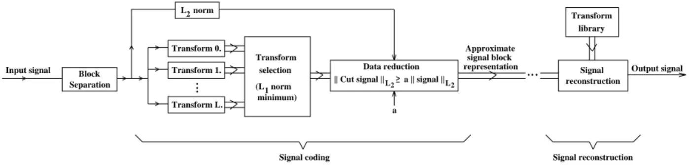
1.5 Overcomplete signal representations ...25

1.5.1 Introduction...26

1.5.2 Overcomplete signal representation ...27

1.5.3 Recursive Overcomplete Signal Representation and Compression...28

1.5.4 Illustrative examples ...29

1.6 Uncertainty handling in non-linear systems ...34

1.6.1 Introduction...34

1.6.2 Uncertainty representation based on probability theory ...35

1.6.3 Uncertainty representation based on fuzzy theory...37

1.6.4 Mixed data models...40

1.6.5 Qualification of results in case of mixed data models ...45

PART II NEW METHODS IN DIGITAL IMAGE PROCESSING... 47

2.1 Introduction...47

2.2 Corner detection...47

2.2.1 Introduction...48

2.2.2 Noise Elimination ...49

2.2.3 Gaussian Smoothing ...50

2.2.4 Determination of the local structure matrix...52

2.2.5 The new corner detection methods ...52

2.2.6 Comparison of different corner detection methods ...55

2.3 “Useful” information extraction ...58

2.3.1 Introduction...58

2.3.2 Surface smoothing ...59

2.3.3 Edge detection ...59

2.3.4 The new primary edge extraction method ...60

2.4 High Dynamic Range (HDR) Imaging ...62

2.4.1 Introduction...62

2.4.2 Background...63

2.4.3 Anchoring theory ...64

2.4.4 Fuzzy set theory based segmentation of images into frameworks ...65

2.4.5 Anchor based new algorithms ...66

2.4.6 A new Tone mapping function based algorithm...68

2.4.7 Illustrative example ...69

2.5 Multiple exposure time HDR image synthetization ...70

2.5.1 Introduction...71

2.5.2 Measuring the Level of the Color Detail in an Image Region...71

2.5.3 HDR image synthesization ...72

2.5.4 Illustrative example ...75

PART III AUTOMATIC 3D RECONSTRUCTION AND ITS APPLICATION IN VEHICLE SYSTEM DYNAMICS... 77

3.1 Introduction...77

3.2 Matching the corresponding feature points in stereo image pairs ...78

3.2.1 Linear solution for the fundamental matrix ...80

3.2.2 New similarity measure for image regions ...81

3.2.3 Automatic image point matching...82

3.2.4 Experimental results ...82

3.3 Camera Calibration by Estimation of the Perspective Projection Matrix...84

3.4 3D reconstruction of objects starting of 2D photos of the scene ...86

3.4.1 3D reconstruction...86

3.4.2 Experimental results ...87

3.5 The intelligent car-crash analysis system ...88

3.5.1 Introduction...88

3.5.2 The concept of the car-crash analysis system...89

3.5.3 Determination of the direction of impact, the absorbed energy and the equivalent energy equivalent speed ...89

3.5.4 Experimental results ...92

PART IV GENERALIZATION OF ANYTIME SYSTEMS, ANYTIME EXTENSION OF FUZZY AND NEURAL NETWORK BASED MODELS... 97

4.1 Introduction...97

4.2 Anytime processing ...99

4.2.1 Alternatives of anytime processing ...100

4.2.2 Measurement of speed/accuracy characteristics (performance profiles)...101

4.2.3 Compilation of complex anytime algorithms ...102

4.2.4 New compilation methods ...104

4.2.5 Open questions...109

4.3 Singular Value Decomposition...110

4.4 Exact and Non-Exact Complexity Reduction of Fuzzy Models and Neural Network Based on SVD...112

4.4.1 Reduction of PSGS fuzzy rule-bases with SVD...112

4.4.2 Reduction of near PSGS fuzzy rule-bases with SVD ...117

4.4.3 Reduction of Takagi-Sugeno fuzzy models with SVD...121

4.4.4 Reduction of generalized neural networks with SVD ...124

4.5 Transformation of PSGS fuzzy systems to iterative models ...131

4.5.1 SVD based transformation of PSGS fuzzy systems to iterative models ...131

4.5.2 Error estimation ...133

4.6 Anytime Modeling: Complexity Reduction and Improving the Approximation ...134

4.6.1 Reducing the complexity of the model ...134

4.6.2 Improving the approximation of the model ...135

4.7 Anytime Control Using SVD Based Models...139

4.8 Anytime Development Environment and the ATDL Anytime Description Language...140

4.8.1 Anytime Development Tool ...140

4.8.2 Anytime Library ...142

4.8.3 Description of anytime systems: the new ATDL meta-language ...143

4.9 Conclusion ...144

PART V OBSERVER BASED ITERATIVE SYSTEM INVERSION... 145

5.1 Introduction...145

5.2 Inverse fuzzy models in measurement and control...146

5.3 Observer based iterative inversion...148

5.4 Genetic algorithms for fuzzy model inversion ...150

5.4.1 The multiple root problem ...150

5.4.2 Genetic algorithm based inversion ...150

5.4.3 The new globally convergent hybrid inversion method ...151

5.5 Fuzzy inversion in anytime systems ...152

5.6 Inversion of Neural Network Models ...152

5.7 Illustrative examples ...153

5.8 Conclusions...156

PART VI SUMMARY OF THE NEW RESULTS ... 157

Result 1: New methods in digital signal processing and data representation ...157

Result 2: New methods in digital image processing ...157

Result 3: Automatic 3D reconstruction and its application in intelligent vehicle system dynamics ...158

Result 4: Generalization of anytime systems, anytime extension of fuzzy and neural network models...159

Result 5: Observer-based system inversion ...159

REFERENCES ... 160

Part I...160

Part II ...162

Part III ...163

Part IV ...164

Part V ...166

PUBLICATIONS OF THE AUTHOR ... 168

Books, book chapters ...168

Journal papers ...168

Conference papers published in proceedings...170

Introduction and objectives

Nowadays, engineering science tackles problems of previously unseen spatial and temporal complexity. In solving engineering problems, the processing of the information is performed typically by model-based approaches which contain a representation of our knowledge about the nature and the actual circumstances of the problem in hand. These models are part of the (usually computer based) problem solving procedure. Up to recently, classical problem solving methods proved to be entirely sufficient in solving engineering problems, however in our days traditional information processing methods and equipment fail to handle the problems in a large number of cases. It became clear that new ideas are required for the specification, design, implementation, and operation of sophisticated systems.

Fortunately however, parallel with the complexity explosion of the problems in focus, we can witness the appearance of increased computer facilities, and also new, fast and intelligent techniques. As a consequence of the new challenges, not only the new problems, arising from the increasing complexity have to be solved, but also new requirements, formulated for information processing, have to be fulfilled. The previously accepted and used (classical) methods only partially cope with these challenges.

Due to the growth of the amount of available computational resources, more and more complex tasks can/are to be addressed by more and more sophisticated solutions. In many cases, processing has to be solved on-line, parallel with information acquisition or operation. Many processes should run with minimized human interaction or completely autonomously, because the human presence is impossible, uncomfortable, or it is against human nature. Furthermore, no matter how carefully the design of the operation/processing scheme is done, we can not avoid changes in the environment;

concerning the goals of the processing, one also have to deal with time/resource insufficient situations caused by failures or alarms. It is an obvious requirement that the actual processing should be continued to ensure appropriate performance in such cases.

What previously was called ‘processing’ became ‘preprocessing’, giving place to more advanced problems. Related to this, the aims of the newly developed preprocessing techniques have also changed. Besides the improvement of the performance of certain algorithms, a new requirement arose: the introduced methods have to give more support to the ‘main’ processing following them.

In signal processing, image processing, and computer vision this trend means that the previous processing tasks like noise smoothing, feature extraction (e.g. edge and corner detection), and even pattern recognition became part of the preprocessing phase and processing covers fields like 3D modeling, medical diagnostics, or the automation of intelligent methods and systems (automatic 3D modeling, automatic analysis of systems/processes etc.).

This work deals with the problems outlined above and tries to offer appropriate computational tools in modeling, data representation, and information processing with dedicated applications in the fields of measurement, diagnostics, signal and image processing, computer vision, and control.

The special circumstances of online processing and the insufficient, unambiguous, or even lacking knowledge call for fast methods and techniques, which are flexible with respect to the available amount of resources, time, and information, i.e. which are able to tolerate uncertainty and changing circumstances. Thus, the focus of this work is on methods of this type.

Part I addresses the topic of signal processing and data representation. New fast recursive transformed-domain transformations, filter and filter-bank implementations are presented as replies to the complexity challenges. Besides complexity reduction, and the decrease of processing delay, the introduction of soft computing (e.g. fuzzy and anytime) techniques offers flexible and robust

operational modes. The newly initiated concepts and techniques however require reconsideration of data and error representation. This question is also briefly addressed here and the usage of some new data and error models is analyzed.

In Part II, new problems of image processing are studied. Different aspects of information enhancement, like corner detection, useful information extraction, and high dynamic range imaging are investigated. The proposed novel tools usually include improvements achieved by fuzzy techniques. Besides being very advantageous from the automation point of view, they may also give an efficient support to the increase of the reliability of further processing.

Based on the results of the previous chapter, Part III presents new methods in computer vision together with the basic elements of a possible intelligent expert system in car-crash analysis.

Autonomous camera calibration and 3D reconstruction are solved with the help of recent results of epipolar geometry and fuzzy techniques. The proposed analyzer system is able to autonomously determine the 3D model of a crashed car and estimate speed and direction of the crash currently in case of one car hitting a wall.

Part IV introduces the generalized concept of anytime processing. Fuzzy and neural network based models are very advantageous if the processing has to be done under incomplete and imperfect circumstances, or if it is crucial to keep computational complexity low. Here, the usage of such models is investigated in anytime systems. With the help of (Higher Order) Singular Value Decomposition based complexity reduction, certain fuzzy and neural network models are extended to anytime use and new error bounds are determined for the non-exact models. In case of Product- Sum-Gravity-Singleton fuzzy systems, a novel transformation opening the way for iterative evaluation is also derived.

Part V deals with observer based fuzzy and neural network model inversion. Model inversion has a significant role in measurement, diagnostics, and control, however until recently, the inversion of fuzzy and neural network model could be solved only with strong limitations on the model. The presented new concept can be applied in more general circumstances and the condition of low complexity, global convergence can also be met.

Part I New Methods in Digital Signal Processing and Data Representation

Signal processing is involved in almost all kinds of engineering problems. When we measure, estimate, or qualify various parameters and signals during the monitoring, diagnostics, control, etc., procedures, we always execute some kind of signal processing task. The performance of measurement and signal processing has usually a direct effect on the performance of the whole system and vice versa, the requirements of the monitoring, diagnostics, or control raise demands in the measurement and signal processing scheme.

The recent development of modern engineering technology, on one hand lead to new tools like model based approaches, computer based systems (CBS), embedded components, dependability, intelligent and soft computing based techniques offering new possibilities; while on the other hand new problems like complexity explosion, need for real-time processing (very often mission-critical services), changing circumstances, uncertain, inaccurate and insufficient information have to be faced. The current situation of engineering sciences is even more complex due to the fact that in very complex systems various modeling approaches, expressing different aspects of the problem, may be used together with a demand for well orchestrated integration. The price to be paid for integration is that the traditional metrological concepts, like accuracy and error have to be reconsidered and in many cases they are no more applicable in their usual approved sense. Furthermore, the representation method of the uncertainty and the error must be in harmony with both the modeling and information processing method. They also need to be uniform or at least “interpretable” by other representation forms. All these lead to the consideration of new, fast and flexible computational and modeling techniques in measurement and signal processing.

This chapter deals with new methods in the fields of digital signal processing and data representation, which offer solution to some of the above outlined problems.

1.1 Introduction

In signal processing the model of a system in question serves as a basis to design processing methods and to implement them at the equipment level. In case of complex signal processing analytical models, it is not enough to obtain a well defined numerical optimal information processing. The complexity of the problem manifests itself not only in the (possibly huge) amount of tasks to be solved or as a hierarchy of subsystems and relations: often several modeling approaches are needed to grasp the essence of the modeled phenomenon. Analytical models rarely suffice. Numerical information is frequently missing or it is uncertain, making place for various qualitative or symbolic representation methods.

The subject of Part I is a topics with increasing actuality. New methods of signal processing are introduced and their role in overcoming several aspects of the above problems is investigated.

Because of the nature of the problems and because we usually need online processing to solve the tasks in hand, only fast algorithms of digital signal processing and new soft computing based methods are concerned. The idea of using fuzzy logic and neural networks combined with other tools like anytime algorithms comes from many other fields of research where similar problems have appeared. It appeared natural to explore and adopt the solutions.

In the fields of Artificial Intelligence (AI), Soft Computing (SC), and Imprecise Computations (IC), numerous methods have been developed, which address the problem of symbolic, i.e. non- numerical information processing and a rational control of limited resources. They may offer a way in signal processing as well when classical methods fail to solve the problems [S46], [S48].

Besides the “basic” method of SC and IC, a major step was done by the introduction of anytime models and algorithms that offer an on-line control over resources and the trade-off between accuracy and complexity (i.e. the use of resources).

The concepts and algorithms presented in this part are advantageous from complexity point of view however the reduction of complexity most often runs parallel with the decrease of accuracy that makes necessary in certain applications to change from one model to another according to the actual situation. The use of different models within one system initiates further difficulties.

We can not forget that results (outputs) produced by different representation methods have to be comparable, convertible, interpretable by each other. This leads to a huge number of open questions not fully answered yet.

The chapter is organized as follows: In Section 1.2 a new concept of multisine synthesis and analysis via Walsh-Hadamard transformation is presented. It is a low complexity, symmetrical, highly parallel structure-pair, also decreasing such disadvantageous effects like picket fence and leakage. In Section 1.3 the usage of fast sliding transforms is discussed in transform-domain adaptive filtering. The resulted reduction of the delay is also analyzed. Section 1.4 is devoted to a novel, low complexity implementation of Fourier transformation, resulting in anytime operational mode, which is able to produce good quality frequency and amplitude estimations of multisine signal components as early as the quarter of the signal block. In Section 1.4 a new overcomplete signal representation is proposed for representing non-stationary signals. Finally, in Section 1.5 new problems of data and uncertainty representation, arising from the non- linearity of systems and from the use of non-conventional modeling methods, are investigated together with some possible solutions offered.

1.2 Multisine synthesis and analysis via Walsh-Hadamard transformation

In this section, we present a new multisine synthesizer and analyzer based on a special filter- bank pair. The new tool can efficiently be utilized for solving system identification problems.

The filter-banks are fast indirect implementations of the inverse discrete (IDFT) and discrete Fourier Transformation (DFT) algorithms providing low computational complexity and high accuracy. The proposed structures are based on the proper combination of polyphase filtering and the Walsh-Hadamard (WHT) Transformations. The inherent parallelism of these structures enables very high speed in practical implementations and the use of several parallel A/D, D/A converters.

1.2.1 Introduction

The classical solutions in digital signal processing offer very well established methods for the frequency-domain signal representation like the discrete Fourier Transformation (DFT) and its fast algorithm the fast Fourier transformation. [1], [2]. However, we have to face serious limits due to the contradictory requirements of magnitude and frequency resolution. To reduce these problems the application of multisine perturbation signals came into focus [3] recently.

Another disadvantageous aspect of the widely used FFT techniques is that they are operated block-oriented, (i.e. the algorithm processes whole blocks of data). Thus, they do not directly support real-time signal processing, which also has become an important claim in this field.

Using the classical recursive DFT methods [1] the real-time processing can be solved with a higher computational burden relative to the FFT. Later, the classical version based on the Lagrange structure was replaced by an observer structure [4], [5] however, computational

complexity remained the same.

Recently a fast implementation of the recursive DFT has been developed [6] which combines the idea of polyphase filtering [7] and the FFT; it is based on the decomposition of a larger size single-input multiple-output (SIMO) DFT filter-bank into proper parallel combination of smaller ones. Its computational complexity is in direct correspondence with the FFT and besides, its polyphase nature provides additional advantages in parallelization.

Using this structure, a fast adaptive Fourier analyzer [8] can be derived and by applying recursive building blocks within the structure a recursive DFT with fading memory can also be implemented [9]. These have real importance in system identification problems where periodic, multi-frequency perturbation signals are applied.

In this Section, a dedicated novel structure pair is presented for the efficient solution of the above described problems. In Subsection 1.2.2 the application of synchronized signal synthesis and analysis is proposed while in section 1.2.3 the new fast recursive synthesis and analysis structure based on the Walsh-Hadamard Transformation will be detailed. Subsection 1.2.4 is devoted to the extension towards multiple parallel running A/D converters.

1.2.2 Synchronized synthesis and analysis ([S6], [S7], [S34], [S35])

In multisine measurements the perturbation signal of the system to be identified is a multisine signal and the amplitudes and phases of the harmonic components of the response are to be measured. The accuracy of the identification depends on the accuracy of the determination of the input/output ratio of the components. If we synchronize the synthesis and analysis of the harmonic components then the systematic error of the DFT/FFT methods can be eliminated. The synchronization can be solved through the use of a joint pair of signal synthesizer and analyzer.

Fig. 1.1 shows the block diagram of the multisine measuring procedure.

N-1 N-1

X 1 X₀ X

Y Y Y 1 0 Analyzer

Unknown system

Evaluation Control Synthesizer

Fig. 1.1 Block diagram of the multisine measuring setup

The synthesizer and analyzer units contain the signal conditioning circuits and the D/A and A/D converters, respectively. The synthesizer generates a multisine input signal for the system with components in given frequency positions and with maximized quasi-uniform amplitudes. This can be optimized through the appropriate setting of the phase positions [3]. The analyzer is the inverse of the synthesizer: its channels are “tuned” to the components of the multisine signal.

The transfer function is determined by the ratio of the complex output/input values. This is evaluated by the common control unit.

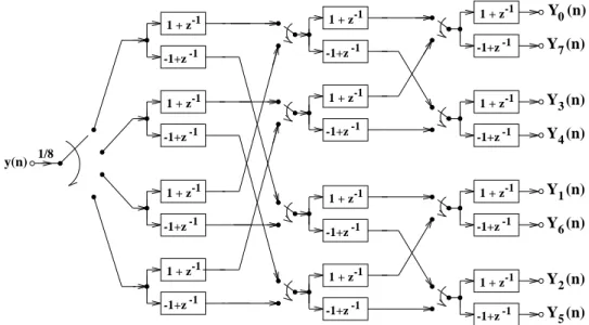
1.2.3 Synthesis and analysis via Walsh-Hadamard transformation ([S2], [S6], [S33]) The block diagram of the proposed synthesizer is given in Fig. 1.2. It is a multiple input single output (MISO) system which can generate arbitrary periodic waveforms. It operates like a parallel to serial converter, i.e. it has a nonzero parallel input in every N-th step and generates a sequence of N samples corresponding to the actual input. If this input is repeated in every N-th step the output will be a periodic waveform. The overall structure implements a complete weighted set of Walsh-Hadamard basis sequences in an efficient form with a complexity

corresponding to that of the fast algorithms. It is important to note that the input signal is the Walsh-Hadamard representation of the sequence to be generated with an accuracy depending only on the accuracy of the weights since within the structure only additions and subtractions are to be performed. The output is obtained via a demultiplexer which can be applied to a D/A converter.

As an example Fig. 1.3 shows a single sinusoid waveform generated using the above method.

The input values of the Walsh-Hadamard synthesizer can be easily calculated as the Walsh- Hadamard transform of the time-sequence to be generated. Let us denote the vector of this sequence by x=[x(0), x(1),...,x(n-1)]^T , and the N*N transformation matrix by W. The N vectors to be applied in every N-th step at the input of the synthesizer are given by X=Wx.

The block diagram of the analyzer structure is given in Fig. 1.4. It is in complete correspondence with the synthesizer and can be considered as a serial to parallel converter system maximally decimated at its output if necessary. The different channels calculate the Walsh-Hadamard coefficients corresponding to the last N input samples. The complexity remains the same as for the generation.

If the output of the synthesizer is connected directly to the input of the analyzer then after N

x(n) 1 - z

1 + z^-1 -1

1 + z 1 - z -1 -1 1 - z 1 + z^-1

-1

1 + z-1 1 - z^-1 1 - z

1 + z^-1 -1

1 - z 1 + z^-1

-1

1 - z 1 + z^-1

-1

1 - z 1 + z^-1

-1

X (n) X (n)₆

1

X (n) X (n)₄

3

X (n) X (n)₇

0

X (n) X (n)₅

2

1 + z 1 - z -1 -1 1 - z 1 + z^-1

-1 1 - z 1 + z^-1

-1

1 + z-1 1 - z^-1

Fig. 1.2 Block diagram of the Walsh-Hadamard synthesizer for N=8

0 10 20 30 40 50 60 70 80

−1

−0.8

−0.6

−0.4

−0.2 0 0.2 0.4 0.6 0.8 1

steps

amplitude

(a) input signal, (b) output of the WHD synthetizer

(a)

(b)

Fig. 1.3 Single sinusoid waveform generated using WHT-synthesizer: (a) desired signal; (b) output signal

steps its output values will equal the Walsh-Hadamard transform components, i.e. the components of X. If there is a system to be identified in between, then we can characterize the unknown system by the corresponding channel inputs X and outputs Y of the synthesizer and the analyzer, respectively. The widely used frequency domain characterization of the system, however, requires some additional computations. On the input side the vector of the complex Fourier components XF can be calculated as

X V X W F x F

X_F = = ⁻¹ = (1.1)

where F stands for the N*N discrete Fourier Transformation (DFT) matrix, while at the output of the analyzer

-1

-1

-1 1 + z

1 + z -1

1 + z

1 + z

-1 1 + z

-1

-1

-1 1 + z 1 + z 1 + z

-1 -1 -1 -1 1 + z

1 + z

1 + z

1 + z -1+z

-1+z

-1+z

-1+z -1 -1 -1 -1

1/8

-1+z

-1+z

-1+z

-1+z -1

-1

-1

-1

-1+z

-1+z

-1+z

-1+z -1

-1

-1

-1 y(n)

6 1 4 3 7 0

5 2

Y (n)

Y (n) Y (n)

Y (n) Y (n)

Y (n) Y (n) Y (n)

Fig. 1.4 Block diagram of the Walsh-Hadamard analyzer for N=8 Y

V Y W F y F

Y_F = = ⁻¹ = . (1.2)

The stationary behavior of the system to be identified can be characterized by the transfer values derived as the ratio of the corresponding components of YF and XF as the transients of the overall system die out. It is important to note that the results will be available at the end of a complete sequence of N samples, i.e. in every N-th step.

Based on (1.1), the practical measurements start with the specification of the proper multisine signal. This is performed by setting the proper initial magnitude and phase via the components of XF (see [3]). The next step is the calculation of the vector X=V^-1XF, which is directly used in the signal generation (see Fig. 1.2). Finally, the output of the analyzer (see Fig. 1.4) should be introduced into (1.2) to get the corresponding sine-wave parameters. The measurement setup described above is a finite impulse response FIR filter-bank which performs a sliding-window mode of operation and therefore its outputs characterize always the last block of N samples, i.e.

each channel of the bank can be considered as a “moving-average” filter. If we consider the effect of the sliding window also for XF then we can extend the method to get a new measurement in every step.

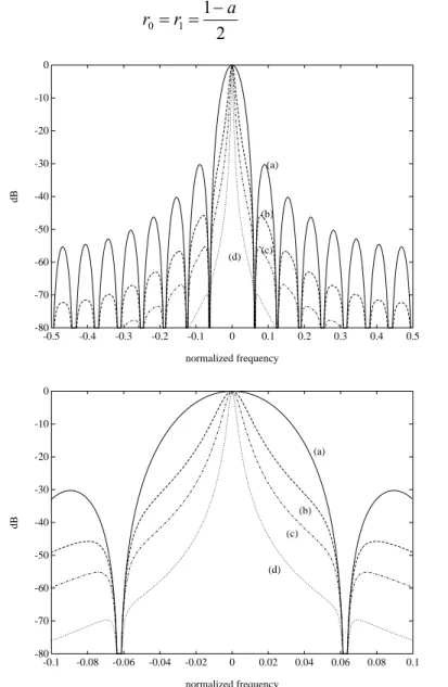
In practical measurements the presence of noise is unavoidable If we model the noise effects as an additive white noise input to the analyzer having variance σ², then this variance will be reduced to σ²/N in every channel. Further improvement can be achieved if we introduce the fading memory effect described in [11] and [12]. The characterization of this effect can be given as

1 1

1 1

1 1

−

−

−

−

−

−

−

z az

z N

a

N N

, (1.3)

where the poles located at the positions determined by the N-th roots of 0 < a < 1 are responsible for further noise reduction. The effects of these poles can be illustrated with the corresponding magnitude characteristics (see Fig. 1.5 for different a values). The extension of the Walsh- Hadamard transformer to such a fading memory version can be solved with the application of simple second-order recursive blocks. If the first stage of the structure in Fig. 1.4 consisting of N/2 2*2 Walsh-Hadamard transformers is realized using e.g. the second-order blocks of Fig. 1.6 with

2 1

1 0

r a

r = = − (1.4)

-80 -70 -60 -50 -40 -30 -20 -10 0

-0.5 -0.4 -0.3 -0.2 -0.1 0 0.1 0.2 0.3 0.4 0.5

(a)

(b)

(d) (c)

normalized frequency

dB

-80 -70 -60 -50 -40 -30 -20 -10 0

-0.1 -0.08 -0.06 -0.04 -0.02 0 0.02 0.04 0.06 0.08 0.1 (a)

(b) (c)

(d)

normalized frequency

dB

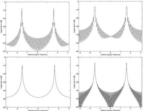
Fig. 1.5 Magnitude characteristics of the filter-banks with different a > 0 parameters: (a) a=0, (b) a=0.4, (c) a=0.6, and (d) a=0.8.

then the overall structure will produce the modified performance described by (1.3). The prize to be paid for this improvement in noise reduction is the increase of the measurement time, since the poles introduced will cause longer transients. As simple example Fig. 1.7 shows the simulated measurement results of a 5th-order Butterworth low-pass filter. After 10 complete periods of the multisine input the measurement results show very good coincidence with the calculated theoretical values.

z^-1

z^-1

0(n) Y

(n) Y₁

r₁ r₀

r₀=r₁=1/2

x(n)

-1 -1

Fig. 1.6 Second-order recursive filter block

0 0.05 0.1 0.15 0.2 0.25 0.3 0.35 0.4 0.45 0.5

−100

−90

−80

−70

−60

−50

−40

−30

−20

−10 0

relative frequency

magnitude response [dB]

0 0.05 0.1 0.15 0.2 0.25

−3

−2.5

−2

−1.5

−1

−0.5 0

relative frequency

magnitude response [dB]

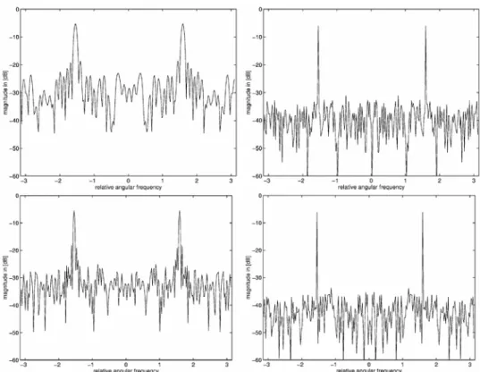
Fig. 1.7 Simulation results of a 5th-order Butterworth low-pass filter: (-) theoretical results, (o) simulated values

1.2.4 Multiple A/D converters within the fast polyphase transformed domain analyzer [S33]

A more detailed block diagram of the complete measuring system shown in Fig. 1.1 is given in Fig. 1.8. This system can be considered as a highly parallel network analyzer, i.e., it is devoted to problems where perturbation signals are to be applied and the system to be measured can be considered as linear. The multisine synthesizer and the signal analyzer operate synchronously together with the D/A and A/D converters. If frequency transposition circuits are also applied then a synchronized “carrier-band” analysis, i.e., “zoom” analysis is also possible. Concerning errors within the system: if we neglect the quantization errors of the digital signal processing parts then only the side-effects of the D/A and A/D conversions and the frequency transpositions are to be considered. Fortunately, frequency mismatch problems can be completely avoided since frequency transpositions can share common frequency reference. On the other hand, the magnitude and phase errors of these circuits can be “measured” by the system itself, since the output of the signal generator can be directly analyzed and the calculated difference of the multisine signal parameters can directly serve for correction. If the D/A and A/D converters share common voltage reference then the system is capable to calibrate itself automatically relative to this reference.

Nowadays the accuracy of measurement systems can be considerably improved by the direct utilization of signal processing techniques. The available DSP processors can provide also good speed performance. Speed and accuracy, however, are contradictory requirements in measurements. As far as A/D conversion is concerned flash converters can operate at very high speed, but their resolution is not acceptable. Sigma-delta A/D converters provide excellent

Fig. 1.8 Detailed block diagram of the multisine measuring system

resolution and accuracy, but at the prize of low conversion rate. For high resolution (>16 bits) measurements a possible alternative can be the application of parallel sigma-delta converters at the input of the polyphase DFT/WHT analyzer (see Fig 1.4) since its internal processing elements operate at a much lower rate. The delay caused by the converters can be easily compensated either in the phase of the generated signal or as a correction during self-calibration.

If the signal processing part of the system would limit the speed of operation then the proposition in the previous section may help where signal generation and analysis is performed via the computationally extremely efficient Walsh-Hadamard transformation.

1.3

Fast sliding transforms in transform-domain adaptive filtering

Transform domain adaptive signal processing proved to be very successful in numerous applications especially where systems with long impulse responses are to be evaluated. The popularity of these methods is due to the efficiency of the fast signal transformation algorithms and that of the block oriented adaptation mechanisms. In this section the applicability of the fast sliding transformation algorithms is investigated for transform domain adaptive signal processing. It is shown that these sliding transformers may contribute to a better distribution of the computational load along time and therefore enable higher sampling rates. It is also shown that the execution time of the widely used Overlap-Save and Overlap-Add Algorithms can also be shortened. The prize to be paid for these improvements is the increase of the end-to-end delay which in certain configurations may cause some degradation of the tracking capabilities of the overall system. Fortunately, however, there are versions where this delay does not hurt the capabilities of the adaptation technique applied.

1.3.1 Introduction

In recent years, transform-domain adaptive filtering methods became very popular especially for those applications where filters with very long impulse responses are to be considered [13]. The basic idea is to apply the fast Fourier Transformation (FFT) for signal segments and to perform adaptation in the frequency domain controlled by the FFT of an appropriate error sequence.

There are several algorithms based on this approach [13] and further improvements can be achieved ([14]). The formulation of the available methods follows two different concepts. The first one considers transformations as a “single” operation to be performed on data sequences (block-oriented approach), while the other emphasizes the role of multirate analyzer and synthesizer filter-banks.

In this section, using some former results concerning fast sliding transformation algorithms ([6], [S33]) a link is developed which helps to identify the common elements of the two approaches.

The fast sliding transformers form exact transformations, however, operate as polyphase filter- banks. These features together may offer further advantages in real-time applications, especially

when standard DSP processors are considered for implementation.

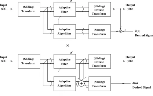
There are two major configurations for transform-domain adaptive filtering (see Fig. 1.9). First let us consider standard (not sliding) transformers. Here transformers perform a serial to parallel conversion while inverses convert to the opposite direction. Adaptation is controlled by the transformed input and error signals once for each input block, i.e. decimation is an inherent operation within these algorithms. At the same time, investigations related to the block-oriented approach rarely consider real-time aspects of signal processing. It is typically supposed that sampling frequency is relatively low compared to the computational power of the signal processors and therefore, if a continuous flow of signal blocks must be processed, the block- period is enough to compute the transformations and the filter updating equations. Moreover, in the case of the widely used Overlap-Save and Overlap-Add methods (see e.g. [13] and Subsection 1.3.4) filter updating requires further transformations, therefore further computational power is needed.

Adaptive Filter Transform

(Sliding) (Sliding)

Inverse Transform

y(n) Output x(n)

Input

Transform (Sliding) Adaptive

Algorithm

-

+ d(n)

Desired Signal

y(n) Output Adaptive

Filter Transform

(Sliding) (Sliding)

Inverse Transform x(n)

Input

Transform (Sliding) Adaptive

Algorithm (a)

d(n) Desired Signal +

-

(b)

Fig. 1.9 Frequency-domain adaptive filter configurations

Filter-bank and consequently fast sliding transformation techniques do not offer extra savings in computations however they may provide a much better distribution of the computational load with time. This means that potentially they give better behavior when real-time requirements are to be met. This section present a new combined structure having advantageous computational complexity and load features. The section is organized as follows: Subsection 1.3.2 describes the basic idea of the fast sliding transforms while Section 1.3.3 is devoted to review the concepts of transform domain adaptive filtering. The new results of the section are introduced in 1.3.4 where the combined structure is characterized.

1.3.2 Fast sliding transformations

Recently a fast implementation of the recursive Discrete Fourier Transformation DFT has been proposed [6] which combines the idea of polyphase filtering and the Fast Fourier Transformation (FFT) algorithm. Figs. 1.10 and 1.11 show the analyzer and the synthesizer DFT filters, respectively. The operation can be easily understood if we observe that e.g. the analyzer at its input follows the decimation-in-time, while at its output the decimation-in-frequency principle. The computational complexity of these structures is in direct correspondence with that of the FFT and its parallel nature provides additional advantages in parallelization.

C O M P E N S A T I O N

X (n)0

X (n)2 X (n)3 X (n)4 X (n)5 X (n)6 X (n)7 X (n)1 2-point

DFT 2-point DFT

2-point DFT 2-point DFT

2-point DFT

2-point DFT

2-point DFT

2-point DFT x(n)

l=0

l=1

m=0

m=1

m=2

m=3

m=0

m=1

m=2

m=3 0

2

1 3

0 2

1 3

0 4

1 5

2 6

3 7 N=8

N=4

N=4

CO MP EN SA TI ON

CO MP EN SA TI ON

8-point 4-point DFT

DFT

4-point DFT 2-point

2-point 2-point

2-point

l=1 l=0 l=1 l=0

DFT

DFT DFT

DFT

Fig. 1.10 Polyphase DFT analyzer for N=8

E N S A T I O N IDFT

2-point CO

MP EN SA TI ON

N=4

CO MP EN SA TI ON

N=4

P

N=8 0

1 5

2 6

3 7

l=0

l=1 m=1

m=2

m=3 m=0

3 1 0 2 m=1

m=2

m=3 m=0

3 1 0

C 2

O M

X (n)7 X (n) X (n)

6 X (n) X (n) X (n) X (n) X (n)

5 4 3 2 1 0

x(n)

4 2-point

2-point 2-point

2-point

4-point

4-point IDFT

IDFT

IDFT

IDFT IDFT

2-point

IDFT 2-point

IDFT 2-point

IDFT

IDFT IDFT 8-point

l=0

l=1

l=0

l=1

2-point

2-point 2-point

2-point IDFT IDFT

IDFT

IDFT

Fig. 1.11 Polyphase DFT synthesizer for N=8

The analyzer bank can be operated as a sliding-window DFT or as a block-oriented transformer.

The latter one means that the parallel outputs are maximally decimated as it is typical with serial to parallel converters. However, if overlapped data segments are to be transformed, the structure is well suited to support decimation by any integer number. The widely used Overlap-Save Method concatenates two blocks of size N to perform linear convolution and calculates 2N-point FFTs. A 2N-point sliding transformer can easily produce output in every N-th step.

In certain applications it may be advantageous to produce signal components instead of the Fourier coefficients as it is dictated by the definition of the DFT. In this case the filter-bank is a set of band-path filters with center frequencies corresponding to the N-th roots of unity values.

Such DFT filter-banks can easily be derived using the ideas valid for the DFT transformers.

With this DFT filter-bank approach, transform-domain signal processing can have the following interpretation: the input signal to be processed first is decomposed by a filter-bank into components and the actual processing is performed on these components. The modified components enter into a N-input single output filter-bank (the so-called synthesizer bank) which produces the output sequence.

1.3.3 Transform-domain adaptive filtering [S44]

The concept of transform-domain adaptive filtering offers real advantages if adaptive FIR filters with very long impulse responses are to be handled. The first important aspect is the possible parallelization described above achievable using fast transformation algorithms. The second is the applicability of block adaptive filtering: the parallel channels enable decimation and

therefore a coefficient update only once in every N-th step. In the meantime, however, a much better gradient estimate can be derived.

Fig. 1.9 shows two possible forms of frequency-domain adaptive filtering. In the first version adaptation is controlled by the time-domain difference of the filter output and the desired signal.

The adaptive filter performs N multiplications using the N-dimensional weighting vector generated by the adaptive algorithm. From the viewpoint of this section, the adaptation mechanism can be of any kind controlled by an error signal, however, in the majority of the applications the least-mean-square (LMS) algorithm is preferred (see e.g. [13]) for its relative simplicity. Adaptation can be performed in every step however drastic reduction of the computations can be achieved only if the transformer outputs are maximally decimated. The techniques developed for this particular case are the so-called block adaptive filtering methods.

[13] gives a very detailed analysis of the most important approaches. It is emphasized that the classical problem of linear versus circular convolution appears also in this context. This problem must be handled because in the majority of the applications a continuous data flow is to be processed and therefore the dependence of the neighboring blocks can not be neglected without consequences. The correct solution is either the Overlap-Save or the Overlap-Add Method. Both require calculations where two subsequent data blocks are to be concatenated and double-sized transformations are to be performed.

If we consider the system of Fig. 1.9a from timing point of view, it is important to observe that at least two transformations must be calculated within the adaptation loop. If real-time requirements are also to be fulfilled, the time needed for these calculations may be a limiting factor. Moreover, if we investigate more thoroughly e.g. the Overlap-Save Method it turns out that the calculation of the proper gradient requires the calculation of two further transformations, i.e. there are altogether four transformations within the loop. This may cause considerable delay and performance degradation especially critical in tracking non-stationary signals.

The adaptation of the transform-domain adaptive filtering scheme on Fig. 1.9b is controlled by an error vector calculated in the transform-domain. Due to this solution the transformer blocks are out of the adaptation loop, therefore the delay within the loop can be kept at a lower level.

Here the adaptation is completely parallel and is to be performed separately for every “channel”.

The operation executed in this scheme corresponds to the circular convolution which may cause performance degradation due to severe aliasing effects.

In the literature of the analysis filter-banks the so-called sub-band adaptive filters see e.g. [13]

are suggested for such and similar purposes which provide better aliasing suppression at the prize of smaller L<N decimation rates. The fast sliding transformers are in fact efficiently implemented special filter-banks. If they are maximally decimated they suffer from the side- effects of the circular convolution. In order to reduce aliasing the application of L=N/2 can be advised. If the number of the adaptive filter channels is lower than the size of the sliding transformer the standard windowing techniques (see e.g. [1]) can be used for channel-filter design.

1.3.4 Adaptive filtering with fast sliding transformers [S44]

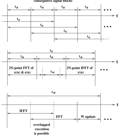
In this subsection the timing conditions of the frequency-domain adaptive filters using the famous Overlap-Save Method are investigated. The block diagram of the method can be followed by Fig. 1.12. The technique is carefully described in [13] therefore here only the most critical elements are emphasized. Other techniques can be analyzed rather similarly.

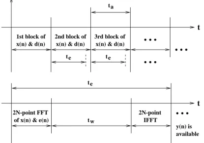
Fig. 1.13 shows the timing diagram of the standard block-oriented solution. Here the acquisition of one complete data block (N samples) is followed by the processing of this data vector. A continuous sequence of data blocks can be processed if the execution time of one block adaptation is less or equal to the corresponding acquisition time (te≤ta). One block adaptation consists of several steps, among them the transformation of the input and the error sequences, respectively (see Fig. 1.9a). The generation of the output sequence requires an additional

0 e

- +

∆

µ 2

X(k)

∆ 0

y(n) Output

d(n) Desired Signal

conj. -

2N-point IFFT

Z^-1

2N-point IFFT Input

x(n)

W(k+1) W(k) X(k)

E(k)

y 2N-point -

FFT

2N-point FFT

2N-point FFT

e(n)

Fig. 1.12 Block diagram of the Overlap-Save Method

transformation. Due to the requirements of the linear convolution all these transformations work on double blocks i.e. on 2N data points. The calculation of the gradient and coefficient update requires two further transformations of this type. A detailed analysis of the steps using the 2N- point transformations shows that none of them is “complete” i.e. some savings in the computations are possible.

With the introduction of the sliding transformers, the acquisition of the input blocks and the processing can be over-lapped, since the sliding transformers can start working already before

ta

te te

t

x(n) & d(n) x(n) & d(n) x(n) & d(n)

1st block of 2nd block of 3rd block of

tw te

IFFT

t

of x(n) & e(n)

2N-point FFT 2N-point

y(n) is available

Fig. 1.13 Timing diagram of the standard overlap-save frequency-domain adaptive algorithms (ta

denotes the acquisition time of one data block of N samples, te stands for the execution time of one block adaptation, and tw is the calculation time of the gradient and the W update). The end-

to-end delay is of N samples

having the complete block. If we permit an end-to-end delay of 2N samples then the processing can be extended for three acquisition intervals (see Fig. 1.14). During the first interval the data acquisition is combined with the transformation, the second can be devoted for finishing the transformation, for updating the coefficient vector and to start the inverse transformation which can be continued in the third interval because the data sampling performed parallel provides the d(n) samples (see Fig. 1.9) sequentially. At the prize of larger end-to-end delay, the execution time can be extended for more blocks, as well.

In the case of the Overlap-Save Method, the gradient calculation consists of an inverse transformation, some simple manipulations and a transformation. Since with the sliding inverse transformation a parallel to serial conversion is performed and the sliding transformer implements a serial to parallel conversion, further overlapping in the execution is possible as it is indicated in Fig. 1.14.

The above considerations can result savings if the granularity of the hardware and software elements of implementation enable smooth distribution of the computational load. If separate hardware units are available for the sliding transformations then the parallelism of the execution can be considerably improved. It is important to note that the precedence conditions of block processing do not support such parallelization: the complete data block must be available for a block-oriented operation like a signal transformation.

To illustrate the achievable gain of using fast transforms here, a comparison is made considering the timing and computational conditions of the two approaches. In the usual implementations of the conventional method, data acquisition and processing are separated in time, i.e. after the arrival of a complete input data block an efficient DSP program calculates the transformed

ta ta ta ta

te

te

te

te

t

consequitive signal blocks

ta

ta ta

te

2N-point IFFT of tw y(n)

t

2N-point FFT of x(n) & e(n)

overlapped execution is possible

tw

W update FFT

IFFT

t

Fig. 1.14 Timing diagrams of a possible frequency-domain adaptive algorithm using sliding transformations. (ta denotes the acquisition time of one data block, te stands for the execution time of one block adaptation, and tw is the calculation time of the gradient and the W update).

The end-to-end delay is of 2N samples

values. The sliding FFT introduced in [6] has the same computational complexity as the traditional algorithm. However, data acquisition and processing overlap in the proposed polyphase filter-bank, therefore calculations start well before the complete block becomes available. There are many ways to characterize the complexity of the FFT, one possible figure can be the number of complex multiplications. This figure for the maximally decimated sliding N-point FFT equals (see [6])

8 1 4 log

1 ₂ +



 



= N N

C , (1.5)

i.e. this figure is one of the possible characterizations. These operations, however, are performed partly during the data acquisition, and the number of complex multiplications, which can not be executed before the arrival of the last sample of the block remains only

( )

2= 2 − . (1.6)

As an example, for N=1024 C1=1793 and C2=502, i.e. the possible time gain due to the overlap can be considerable. Similar figures can be given for other operations, as well.

As a summation of the above investigations we can state that with such techniques further parallelism can be achieved and utilized for applications where higher sampling rates are required. The solutions which follow the scheme of Fig. 1.9b are in good correspondence with some successful multirate filter-bank techniques while the other group related to Fig. 1.9a can significantly be improved. The prize to be paid for the additional parallelism is the increase of the overall end-to-end delay which requires further investigations concerning step-size and stability issues. This can be started following the ideas of [15], where a similar problem was to be solved.

In this section, the term “transform-domain” was used instead of the explicit term “frequency- domain” The reason for this is that all the above developments can be extended for other type of transformations, as well. The application of other transformers may reduce either the computational load or in certain cases they improve the adaptation performance.

1.4 Anytime Fourier Transformation

Anytime signal processing algorithms are to improve the overall performance of larger scale embedded digital signal processing (DSP) systems. The early availability of the amplitude and/or frequency components of digital signals can be very important in different signal processing tasks, where the processing is done on-line, parallel with measurements and input data acquisition. It may offer a possible way for increasing the sampling rate (or the complexity of the tasks to be solved during one sampling period) and also to decrease the delay caused by the necessary information collection for setting the measurement/signal processing scheme.

In this section the concept of anytime Fourier transformation is presented and a new fast anytime fuzzy Fourier transformation algorithm is introduced. The method reduces the delay problem caused by the block-oriented fast algorithms and at the same time keeps the computational complexity on relatively low level. It yields partial results of good quality or estimates before the samples of the period arrive. This is especially advantageous in case of abrupt reaction need and long or possibly infinite input data sequences. As a possible application field, the usage of the presented new method in Adaptive Fourier Analysis of multisine signals is also investigated.

The determination of the frequencies of a multisine signal can be very important at different signal processing tasks, like vibration measurements and active noise control related to rotating machinery and calibration equipment. Adaptive Fourier Analyzers have been developed for