arXiv:1905.11613v1 [math.GT] 28 May 2019
ANTONIO ALFIERI, SUNGKYUNG KANG, AND ANDR ´AS I. STIPSICZ
Abstract. Using the covering involution on the double branched cover ofS3branched along a knot, and adapting ideas of Hendricks-Manolescu and Hendricks-Hom-Lidman, we define new knot invariants and apply them to deduce novel linear independence results in the smooth concordance group of knots.
1. Introduction
Concordance questions of knots has been effectively studied by 4-dimensional topo- logical methods. Indeed, for a knot K in the three-sphere S3 consider the double branched cover Σ(K) of S3 branched along K. If K is a slice knot (i.e. bounds a smoothly embedded disk in the 4-diskD4) then Σ(K) bounds a four-manifoldX hav- ing the same rational homology asD4: thisX can be chosen to be the double branched cover of D4 along the slice disk. The existence of such four-manifold then can be ob- structed by various methods, leading to sliceness obstructions of knots. For example, Donaldson’s diagonalizability theorem applies in case Σ(K) is known to bound a nega- tive definite four-manifold with intersection form which does not embed into the same rank diagonal lattice. This line of reasoning was used by Lisca in his work about slice- ness properties of 2-bridge knots, see [6, 15, 19]. A numerical invariant (in the same spirit) was introduced by Manolescu-Owens [20] utilizing the Ozsv´ath-Szab´o correction term of the unique spin structure of Σ(K).
Different knots might admit diffeomorphic double branched covers, though; for ex- ample, if K and K′ differ by a Conway mutation, then Σ(K) and Σ(K′) are diffeo- morphic. This implies that if K is slice, all slice obstructions coming from the above strategy must vanish forK′ as well. A long-standing problem of this type was whether the Conway knot is slice; it admits a mutant (the Kinoshita-Terasaka knot) which is slice, hence merely considering the double branched cover will not provide sliceness obstruction. (The fact that the Conway knot is not slice has been recently proved by Piccirillo [34], relying on four-dimensional topological methods and results from Khovanov homology.)
The information we neglect in the above approach is that the three-manifold Σ(K) (viewed as the double branched cover ofS3 alongK) comes with a self-diffeomorphism τ, where pairs of points in Σ(K) mapping to the same point ofS3are interchanged byτ. In this paper we introduce modifications of the usual Heegaard Floer homology groups of Σ(K) which take this Z/2Z-action into account, leading to new knot invariants.
Heegaard Floer homology associates to a closed, oriented, smooth three-manifold a finitely generated F[U]-module HF−(Y) (where F[U] is the polynomial ring over the field F of two elements): it is the homology of a chain complex (CF−(Y), ∂) (defined up to chain homotopy equivalence) and the homology naturally splits according to the spinc structures of Y as
HF−(Y) =⊕s∈Spinc(Y)HF−(Y,s).
1
If Y is a rational homology sphere (i.e., b1(Y) = 0) then HF−(Y,s) admits a natural Q-grading, and the graded F[U]-module HF−(Y,s) is a diffeomorphism invariant of the spinc three-manifold (Y,s), while the local equivalence class of (CF−(Y,s), ∂) (for the definition of its notion see Definition 3.2) provides an invariant of the rational spinc homology cobordism class of (Y,s). In this case the local equivalence class of CF−(Y,s) can be characterised by a single rational numberd(Y,s), the Ozsv´ath-Szab´o correction term of the spinc three-manifold (Y,s).
More recently, exploiting a symmetry built in the theory, Hendricks and Manolescu introduced involutive Heegaard Floer homology [11]. The main idea of their construc- tion was that the chain complex CF−(Y) admits a map ι: CF−(Y)→CF−(Y) which is (up to homotopy) an involution, and the mapping cone of the map ι+ id provided HFI(Y), a module over the ring F[U, Q]/(Q2). This group is interesting only for those spinc structures which originate from a spin structure, and provides a new and rather sensitive diffeomorphism invariant of the underlying spin three-manifold. A further ap- plication of the above involution appeared in the work of Hendricks, Hom and Lidman [9], where connected Heegaard Floer homology HF−conn(Y), a submodule of HF−(Y) was defined. This submodule turned out to be a homology cobordism invariant.
Similar constructions apply for any chain complex equipped with a (homotopy) involution. In this paper we will define the branched knot Floer homology of K as HFB−(K) =H∗(Cone(τ#+ id)), where τ: Σ(K) → Σ(K) is the covering involution, τ# is the map induced by τ on the Heegaard Floer chain complex CF−(Σ(K),s0), withs0 the unique spinc structure on Σ(K), and Cone is the mapping cone of the map τ#+ id. (Related constructions have been examined in [10].)
Theorem 1.1. The group HFB−(K), as a graded F[U, Q]/(Q2)-module, is an isotopy invariant of the knot K ⊂S3.
A simple argument shows that, as an F[U]-module, HFB−(K) is isomorphic to F[U](δ(K))⊕F[U](δ(K))⊕A, whereδ(K), δ(K)∈Qand Ais a finitely generated, graded U-torsion module over F[U].
Theorem 1.2. The rational numbersδ(K)andδ(K)are knot concordance invariants.
Adapting the method of [9] for defining new homology cobordism invariants of ratio- nal homology spheres, we define the connected branched Floer homology HFB−conn(K) of a knot K ⊂S3 as follows. Consider a sel-local equivalence fmax: CF−(Σ(K),s0)→ CF−(Σ(K),s0) which commutes (up to homotopy) with τ# and has maximal kernel among such endomorphisms. Then take HFB−conn(K) =H∗(Imfmax).
Theorem 1.3. The module HFB−conn(K) (up to isomorphism) is independent of the choice of the map fmax with maximal kernel, and the isomorphism class of the graded module HFB−conn(K) is a concordance invariant of the knotK.
It follows from the construction that HFB−conn(K) is anF[U]-submodule of HF−(Σ(K),s0).
As a finitely generated F[U]-module, HFB−conn(K) is the sum of cyclic modules, and since it is of rank one, it can be written as
HFB−conn(K) =F[U]⊕HFB−red-conn(K),
where the second summand (the U-torsion submodule) is the reduced connected ho- mology of K.
It is not hard to see that if HF−(Σ(K),s0) = F[U] holds — for example if Σ(K) is an L-space, which is the case if K is a quasi-alternating knot —, then τ# is chain homotopic to id implying
Theorem 1.4. If K is concordant to an alternating (or more generally to a quasi- alternating) knot, then HFB−red-conn(K) = 0.
Somewhat more surprisingly, the same vanishing holds for torus knots (a phenom- enon reminiscent to the behaviour of the extension of the Upsilon-invariant of [25] to the Khovanov setting given by Lewark-Lobb in [17]):
Theorem 1.5. For the torus knot Tp,q we have that HFB−red-conn(Tp,q) = 0.
Lattice homology of N´emethi [21] (through results and computations of Dai-Manolescu [2]
and Hom-Karakurt-Lidman [13]) provides a computational scheme of the above invari- ants for Montesinos (and in particular, for pretzel) knots. The combination of some such sample calculations with the two vanishing results above allow us to show that certain families of pretzel knots are linearly independent from alternating and torus knots in the smooth concordance group. To state the results, let us introduce the fol- lowing notations: letC denote the (smooth) concordance group of knots inS3 andQA (respectively T) those subgroups ofC which are generated by all quasi-alternating (re- spectively torus) knots. In addition,QA+T is the subgroup generated by alternating knots and torus knots. The following theorem extends results from [1, 37].
Theorem 1.6. Let K be the connected sum of pretzel knots of the form P(−2,3, q), with q≥7 odd. ThenK is not concordant to any linear combination of alternating or torus knots, i.e. [K] is a nonzero element of the quotient C/(T +QA).
Furthermore, relying on computations from [2, 13], we prove the following.
Theorem 1.7. The pretzel knots {P(−p,2p−1,2p+ 1)|p odd} are linearly indepen- dent in the quotient group C/(T +QA). In paricular, Z∞ ⊂ C/(T +QA).
The paper is organized as follows. In Section 2 we introduce branched knot Floer homology, and in Section 3 we discuss the details of the definition of the connected Floer homology group HFB−conn(K) of a knot K ⊂ S3. Section 4 is devoted to the proof of the vanishing results above, while in Section 5 we give a way to compute the invariants for Montesinos knots; finally in Section 6 we derive some independence results in the smooth concordance group.
Acknowledgements: We would like to thank Andr´as N´emethi for numerous highly informative discussions. The first and the third author acknoweldges support from the NKFIH Elvonal´ project KKP126683. The second author was partially supported by European Research Council (ERC) under the European Union Horizon 2020 research and innovation programme (grant agreement No 674978).
2. Definition of branched knot Floer homology
Let H = (Σ,α,β, z) be a pointed Heegaard diagram which represents a rational homology sphereY, and letJsbe a generic path of almost-complex structures on theg- fold symmetric product Symg(Σ) (compatible with a symplectic structure constructed in [33]). Heegaard Floer homology [29] assigns to the pair (H, Js) a finitely generated, Q-graded chain complex CF−(H, Js) over the polynomial ring F[U], graded so that degU =−2. This chain complex is defined as the free F[U]-module generated by the intersection point of the Lagrangian toriTα =α1× · · · ×αg and Tβ =β1× · · · ×βg in Symg(Σ), and is equipped with the differential
∂x= X
y∈Tα∩Tβ
X
{φ∈π2(x,y)|µ(φ)=1}
# (M(φ)/R)Unz(φ)·y (1)
where #(M(φ)/R) is the (mod 2) number of points in the unparametrized moduli space M(φ)/R of Js-holomorphic strips with index µ(φ) = 1 representing the ho- motopy class φ ∈ π2(x,y) and nz(φ) is the intersection number of φ with the divi- sor Vz = {z} ×Symg−1(Σ). For more details about Heegaard Floer homology see [28, 29, 30, 31].
For a knotK ⊂S3, let Σ(K) denote the double branched cover ofS3 branched along K. The three-manifold Σ(K) comes with a natural map τ: Σ(K)→Σ(K) (called the covering involution) which interchanges points with equal image under the branched covering map π: Σ(K) → Σ(K)/τ ≃ S3. The fixed point set Fix(τ) = Ke maps homeomorphically toK underπ. As the notation suggests (sinceH1(S3\K;Z)∼=Z), the branched cover Σ(K) in this case is determined by the branch locus K ⊂S3.
Pulling back the Heegaard surface, as well as theα- and the β-curves of a doubly- pointed Heegaard diagramD= (Σ,α,β, w1, w2) representingK ⊂S3we get a pointed Heegaard diagram
HD =
Σ =e π−1(Σ),αe =π−1(α),βe=π−1(β), z =π−1(w1)
of the double branched cover Σ(K). The covering projection π: Σ(K)→S3 restricts to a double branched cover of Riemann surfacesπ|Σe: Σe →Σ with branch set{w1, w2}.
The restriction τ|Σe: Σe →Σ of the covering involutione τ represents the covering invo- lution ofπ|Σe: Σe →Σ, andτ|Σe: Σe →Σ induces a self-diffeomorphism of the symmetrice product
σ: Symg(Σ)e →Symg(Σ)e , (2) leaving Tαe and Tβe, as well as the divisor Vz ={z} ×Symg−1(Σ) invariant.e
Pick a generic path of almost-complex structures Js ∈ J(Symg(Σ)) (satisfying thee usual compatibility conditions with the chosen symplectic form on the symmetric product) and consider the Heegaard Floer chain complex CF−(HD, Js) associated to (HD, Js). Recall that there is a direct sum decomposition of CF−(HD, Js) indexed by spinc structures:
CF−(HD, Js) = M
s∈Spinc(Σ(K))
CF−(HD, Js;s) .
The first (singular) homology group of the double branched cover Σ(K) can be presented byθ+θt, where θ is a Seifert matrix forK. Thus, |H1(Σ(K),Z)|= det(θ+ θ′) = det(K), which is an odd number. In particular, Σ(K) has a unique spin structure s0. We will focus on CF−(HD, Js;s0), the summand of CF−(HD, Js) associated to s0. Note that if the path of almost-complex structures Js ∈ J(Symg(Σ)) is chosene generically, transversality is achieved for both Js and the push-forward σ∗Js (where σ is given in Equation (2)). For such a choice of almost-complex structures we have well-defined Heegaard Floer chain complexes CF−(HD, Js) and CF−(HD, σ∗Js), and we can consider the map
η: CF−(HD, Js)→CF−(HD, σ∗Js) (3) sending a generatorx=x1+· · ·+xg ∈Tαe∩Tβe ⊂Symg(Σ) toe σ(x) =τ(x1)+· · ·+τ(xg).
Lemma 2.1. The mapη is an isomorphism of chain complexes. Furthermore,ηmaps the summand CF−(HD, Js;s0) of the spin structure s0 into itself.
Proof. It is obviously an isomorphisms of free F[U]-modules; indeed, η2 = id since τ is an involution. To see that η commutes with the differential, notice that u7→ τ ◦u
provides a diffeomorphism between the moduli space of Js-holomorphic representa- tives of a homotopy class φ ∈ π2(x,y) and the moduli space of σ∗Js-holomorphic representatives of τ◦φ ∈π2(τ(x), τ(y))).
To show that η preserves the spin structure we argue as follows. According to [29, Section 2.6] the choice of a basepoint z of HD determines a map sz: Tαe∩Tβe → Spinc(Σ(K)) and
CF−(HD, Js;s) = M
sz(x)=s
F[U]·x.
It follows from the definition of sz that τ∗(sz(x)) = sz(τ(x)). Thus if sz(x) =s0, we have that
sz(τ(x)) =τ∗(sz(x)) =τ∗(s0) =τ∗(s0) =τ∗(s0) =sz(τ(x))
proving that sz(τ(x)) is a self-conjugate spinc structure, i.e. spin. The claim now follows from the fact that Σ(K) has a unqiue spin structure.
We defineτ#: CF−(HD, Js;s0)→CF−(HD, Js;s0) as the mapη: CF−(HD, Js;s0)→ CF−(HD, τ∗Js;s0) followed by the continuation map
Φ−Js,t: CF−(HD, τ∗Js;s0)→CF−(HD, Js;s0)
from [29, Section 6], induced by a generic two-parameter familyJs,t of almost-complex structures interpolating between Js and τ∗Js:
τ# = ΦJs,t◦η.
Lemma 2.2. τ#2 ≃id, where ≃ denotes chain homotopy equivalence.
Proof. Consider
Φ−Js,t(x) = X
y∈Tαe∩Tβe
X
{φ∈π2(x,y) |µ(φ)=0}
# MJs,t(φ)
Unz(φ)·y where MJs,t(φ) denotes the moduli spaces of Js,t-holomorphic strips.
Given x∈Tαe∩Tβeone computes η◦Φ−Js,t(x) = X
y∈Tαe∩Tβe
X
{φ∈π2(x,y) | µ(φ)=0}
# MJs,t(φ)
Unz(φ)·τ(y)
= X
y∈Tαe∩Tβe
X
{φ∈π2(x,τ(y)) | µ(φ)=0}
# MJs,t(φ)
Unz(φ)·y
= X
y∈Tαe∩Tβe
X
{φ∈π2(τ(x),y) | µ(φ)=0}
# MJs,t(τ◦φ)
Unz(τ◦φ)·y
= X
y∈Tαe∩Tβe
X
{φ∈π2(τ(x),y) | µ(φ)=0}
# MJs,t(φ)
Unz(φ)·y
= Φ−τ
∗Js,t(τ(x)) , hence the identity η◦Φ−H = Φ−τ
∗H ◦η follows. Thus, τ#2 = Φ−Js,t◦η◦Φ−Js,t ◦η = Φ−Js,t◦Φ−τ
∗Js,t◦η2 = Φ−Js,t◦Φ−τ
∗Js,t ,
where the last identity holds becauseη2 = id (a consequence of the fact thatτ: Σ(K)→ Σ(K) is an involution).
By concatenatingJs,tandτ∗Js,twe obtain a one-parameter family of paths of almost- complex structures describing a closed loop based at the path Js. Since the space of
almost complex structures (compatible with the fixed symplectic structure) is con- tractible, we can find a three-parameter family of almost complex structures Js,t,x
interpolating between the juxtaposition of Js,t and τ∗Js,t, and Js,t,1 ≡ Js. As pointed out in [29, Section 6], a generic choice of Js,t,x produces smooth moduli spaces
MJs,t,x(φ) = [
c∈[0,1]
MJs,t,c(φ) φ∈π2(x,y)
of dimension µ(φ) + 1. These can be used to produce a chain homotopy equivalence HJ−s,t,x(x) = X
y∈Tαe∩Tβe
X
{φ∈π2(x,y) |µ(φ)=−1}
# MJs,t,x(φ)
Unz(φ)·y between Φ−Js,t ◦Φ−τ
∗Js,t and id, concluding the argument.
In summary, for a knotK ⊂S3there is a homotopy involutionτ#: CF−(Σ(K),s0)→ CF−(Σ(K),s0) associated to the covering involutionτ: Σ(K)→Σ(K). In order to de- rive knot invariants from the pair (CF−(H,s0), τ#), we follow ideas from [11] and form the mapping cone of τ#+ id : CF−(Σ(K),s0) →CF−(Σ(K),s0), written equivalently as
CFB−(K) = CF−(Σ(K),s0)[−1]⊗F[Q]/(Q2), ∂cone =∂+Q·(τ#+ id) , where degQ=−1. Recall that CF−(Σ(K),s0) admits an absoluteQ-grading, and τ# preserves this grading, hence CFB−(K) also admits an absolute Q-grading. Taking homology we get the group HFB−(K) =H∗(CFB−(K)), which is now a module over the ringF[U, Q]/(Q2). We call HFB−(K) thebranched Heegaard Floer homology of the knot K ⊂ S3. Now we are ready to turn to the proof of the first statement announced in Section 1:
Proof of Theorem 1.1. The proof is similar to the one of [11, Proposition 2.8]. Indepen- dence from the chosen path of almost-complex structures is standard Floer theory. For independence from the chosen doubly pointed Heegaard diagram ofK, we argue as fol- lows: A doubly pointed Heegaard diagramD= (Σ,α,β, w1, w2) representing the knot K ⊂S3can be connected to any other doubly pointed diagramD′ = (Σ′,α′,β′, w′1, w2′) of K by a sequence of isotopies and handleslides of the α-curves (or β-curves) sup- ported in the complement of the two basepoints, and by stabilizations (i.e., forming the connected sum of Σ with a torusT2 equipped with a new pair of curves αg+1 and βg+1 which meet transversally in a single point). A sequence of these moves lifts to a sequence of pointed Heegaard moves of the pull-back diagrams HD and HD′ with un- derlying three-manifold the double branched cover Σ(K). According to [14] the choice of such a sequence of Heegaard moves yields a natural chain homotopy equivalence ψ: CF−(HD)→CF−(HD′) which fits into the diagram
CF−(HD) τ# //
ψ
CF−(HD)
ψ
CF−(HD′) τ
#′
// CF−(HD′)
(4)
that commutes up to chain homotopy. Let Γ : CF−(HD)→CF−(HD′) be a map realiz- ing the chain homotopy equivalence. Then the mapf: Cone(τ#+ id)→Cone(τ#′ + id) defined by f = ψ+Q·(ψ+ Γ) is a quasi-isomorphism. Indeed, f is a filtered map
with respect to the two step filtration of the mapping cones, and since it induces an isomorphism on the associated graded objects, it is a quasi-isomorphism.
Notice that the mapping cone exact sequence associated to CFB−(K) = Cone(τ#+ id) reads as an exact triangle
HF−(Σ(K),s0) HF−(Σ(K),s0)
HFB−(K)
τ∗+id
j∗
p∗ (5)
in which j∗ preserves the grading, andp∗ drops it by one. In particular, ifτ∗ = id, the horizontal map in the above triangle is zero, and in that case HFB−(K) is the sum of two copies of HF−(Σ(K),s0) (with the grading on one copy shifted by one).
A close inspection of the exact triangle above reveals that, asF[U]-modules, we have HFB−(K) = F[U](δ)⊕F[U](δ+1)⊕(F[U]−torsion) .
We set δ(K) =δ and δ(K) =δ, which (by the above discussion) are knot invariants.
Notice that δ(K), δ(K)∈Q, δ(K)≡δ(K)≡δ(K) mod 2, and δ(K)≤δ(K)≤δ(K), whereδ(K) is the Ozsv´ath-Szab´o correction term of (Σ(K),s0), henceδ(K) is half the Manolescu-Owens invariant ofK introduced in [20].
3. Concordance invariants from (CF−(Σ(K),s0), τ#)
Adapting ideas from [9], the chain complex CF−(Σ(K),s0), equipped withτ#, pro- vides concordance invariants of the knot K as follows. Recall [9, Definition 2.5] re- garding ι-complexes:
Definition 3.1. An ι-complex (C, ι) is a finitely generated, free, Q-graded chain complex C over F[U] together with a chain map ι: C → C where C is supported in degree τ +Z for some τ ∈ Q (multiplication by U drops the Q-grading by two), the homology of the localization U−1H∗(C) = H∗(C⊗F[U]F[U, U−1]) is isomorphic to F[U, U−1] via an isomorphism preserving the relative Z-grading, and ι is a grading preserving, U-equivariant chain map which is a homotopy involution.
We will considerι-complexes up tolocal equivalence (see [9, Definitions 2.6 and 2.7]).
Definition 3.2. A local equivalence f: C → C′ of two ι-complexes (C, ι) and (C′, ι′) is a grading preserving, U-equivariant chain map f: C →C′ such that
• ι′◦f ≃f ◦ι, i.e. the two compositions are chain homotopy equivalent,
• f induces an isomorphismsfloc on the localization U−1H∗(C).
Definition 3.3. Two ι-complexes (C, ι) and (C′, ι′) are locally equivalent if there exist local equivalences f: C → C′ and g: C′ → C. If in addition we have f ◦g ≃id andg◦f ≃id, then (C, ι)and (C′, ι′)arechain homotopy equivalent ι-complexes.
Given an ι-complex (C, ι) we can look at the set Endloc(C, ι) of its self-local equiv- alences f: C → C. This can be partially ordered by defining f g if and only if Kerf ⊂ Kerg. We say that f ∈ Endloc(C) is a maximal self-local equivalence if it is maximal with respect to this ordering. By Zorn’s lemma maximal self-local equivalences always exist. The following lemma summarises the results of [9, Section 3].
Lemma 3.4. Let (C, ι) be an ι-complex. Then
(1) if f ∈Endloc(C, ι) is a maximal self-local equivalence, then ι restricts to a ho- motopy involution ιImf of Imf. Furthermore, (Imf, ιImf) is locally equivalent to (C, ι);
(2) if f, h ∈ Endloc(C, ι) are two maximal self-local equivalences, then there is a chain homotopy equivalence (Imf, ιImf)≃(Imh, ιImh) of ι-complexes;
(3) if (C′, ι′) is an ι-complex locally equivalent to (C, ι) and f ∈Endloc(C, ι), and h ∈ Endloc(C′, ι′) are self-local equivalences then there is a chain homotopy equivalence (Imf, ιImf)≃(Imh, ιImh) of ι-complexes.
Since
H∗(CF−(Σ(K),s0)⊗F[U]F[U, U−1]) = HF∞(Σ(K),s0) =F[U, U−1],
the pair (CF−(Σ(K),s0), τ#) of the Heegaard Floer chain complex of the double branched cover of a knot K ⊂ S3 (equipped with the homotopy involution τ# in- duced by the covering involution) is an ι-complex associated to K. Given a maximal self-local equivalence fmax: CF−(Σ(K),s0) → CF−(Σ(K),s0) we define HFB−conn(K), the connected Floer homology of the knot K ⊂S3 asH∗(Imfmax). As an applica- tion of Lemma 3.4, it is then easy to see that the resulting group is a knot invariant:
Theorem 3.5. The chain homotopy type of Imfmax is independent of the choice of the maximal self-local equivalence fmax∈Endloc(CF−(Σ(K),s0), τ#).
We now turn to the proof of concordance invariance of the groups HFB−conn(K). The following naturality statement will be needed in the proof.
Lemma 3.6. (Ozsv´ath & Szab´o, Zemke,[32, 38]) LetY and Y′ be two three-manifolds equipped with self-diffeomorphismsτ: Y →Y andτ′:Y′ →Y′. Suppose thatW: Y → Y′ is a cobordism and that there exists a self-diffeomorphism T: W → W restricting to τ and τ′ on the two ends of W. Then
τ#′ ◦FW,−t =FW,T− ∗t◦τ#
for every t∈Spinc(W).
Proof of Theorem 1.3. Suppose that K′ ⊂ S3 is concordant to K, i.e. there exists a smoothly embedded annulus C ⊂ S3 ×[0,1] with ∂C =C∩S3 ×[0,1] =K × {1} ∪ K′× {0}. By taking the double branched cover Σ(C) of S3×[0,1] branched along C we get a smooth rational homology cobordism from Σ(K) to Σ(K′). By adapting [8, Lemma 2.1] forn= 2, we get that the four-manifold Σ(C) comes with a distinguished spin structuretrestricting to the canonical spin structure on the two ends. In addition, this spin structure is invariant under the covering involution of the double branched cover Σ(C). Let FC−: CF−(Σ(K),s0) → CF−(Σ(K′),s0) denote the cobordism map induced by (Σ(C),t).
Since Σ(C) is a rational homology cobordism, it follows that FC−: CF−(Σ(K),s0)→CF−(Σ(K′),s0) and
F−C− : CF−(Σ(K′),s0)→CF−(Σ(K),s0),
are local equivalences. (Recall that according to [32] a rational homology cobordism induces an isomorphism on HF∞ = U−1HF−.) The fact thatFC− and F−C− homotopy commute with the homotopy Z/2Z-actions follows from Lemma 3.6 and the fact that (in the notations of that lemma) we have T∗t = t. Then Lemma 3.4 concludes the
argument.
Proof of Theorem 1.2. Let f ∈ Endloc(CF−(Σ(K),s0), τ#) be a maximal self-local equivalence. As a consequence of Lemma 3.4, the chain homotopy type of the mapping cone of the restriction τ#Imf + id : Imf → Imf is a concordance invariant of K. On the other hand,
H∗(Cone(τ#Imf + id)) =F[U]δ(K)⊕F[U]δ(K)+1⊕(F[U]−torsion),
implying the claim.
Since HF−(Σ(K),s0) is of rank one (as anF[U]-module), and fmax is a local equiva- lence, it follows that HFB−conn(K)⊂HF−(Σ(K),s0) is also of rank one. TheU-torsion submodule of HFB−conn(K) is the reduced connected Floer homology of K, and it will be denoted by HFB−red-conn(K).
The following simple adaptation of [9, Proposition 4.6] allows us to prove triviality of HFB−red-conn(K).
Proposition 3.7. HFB−red-conn(K) = 0 if and only if δ(K) =δ(K) =δ(K).
Given a knot K ⊂S3 we denote by −K its mirror image.
Lemma 3.8. For a knot K ⊂S3 we have that δ(K) =−δ(−K)
Proof. The double branched cover of−K is−Σ(K). The argument of [11, Proposition
5.2] provides the claimed identity.
Lemma 3.9. If K =K1#K2 for two knots K1 and K2 ⊂S3 then
δ(K1) +δ(K2)≤δ(K)≤δ(K)≤δ(K1) +δ(K2). (6) Proof. Suppose that Di is a doubly pointed Heegaard diagram for Ki ⊂S3 (i= 1,2).
Then a doubly pointed Heegaard diagram D can be constructed for K by taking the connected sums of Di (along w21 in D1 and w22 in D2). This construction shows that CF−(HD) is the tensor product of CF−(HD1) and CF−(HD2). It then obviously follows that the map ηD of Equation (3) forHD is the tensor product of the similar maps ηD1
and ηD2 for HD1 and HD2. This implies that τD and τD1 ⊗τD2 are chain homotopic maps, from which [12, Proposition 1.3] implies the result.
4. Vanishing results
In some cases HFB−(K) and HFB−conn(K) can be easily determined. As customary in Heegaard Floer theory, these invariants do not capture any new information for al- ternating (or, more generally quasi-alternating) knots. It is a more surprising (and as we will see, very convenient) feature of HFB−conn that it is rather trivial for torus knots as well. In this section we show some vanishing results about the group HFB−conn(K), while the next section provides methods to determine our invariants for Montesinos (and more generally for arborescent) knots. We start with a simple motivating exam- ple.
4.1. An example. Consider the Brieskorn sphere Σ(2,3,7); it can be given as (−1)- surgery on the right-handed trefoil knot T2,3. It is an integral homology sphere with Heegaard Floer homology HF(Σ(2,c 3,7)) = F2(0) ⊕F(−1) and HF−(Σ(2,3,7)) = F[U](−2) ⊕F(−2) in its unique spinc (hence spin) structure, see [26, Equation (25)].
This three-manifold can be presented as the double branched cover of S3 either along the torus knot T3,7, or along the pretzel knot P(2,−3,−7). The two presen- tations provide two involutions on Σ(2,3,7), which potentially provide two different
maps on the Heegaard Floer chain complex. Indeed, let φ1 denote the involution Σ(2,3,7) admits as double branched cover along T3,7 and let φ2 denote the involu- tion it gets as double branched cover alongP(2,−3,−7). Through direct calculation, the actions of these maps on Heegaard Floer homology has been identified in [10, Propositions 6.26 and 6.27].
Theorem 4.1 ([10]). The map (φ1)∗ induces the identity map on HF(Σ(2,c 3,7)) (and hence onHF−(Σ(2,3,7)), while the map(φ2)∗is different from the identity onHF(Σ(2,c 3,7)).
This allows us to compute the invariants HFB−and HFB−connforT3,7andP(2,−3,−7), showing that
• HFB−(T3,7) =F[U](−2)⊕F[U](−3)⊕F(−2)⊕F(−3), or, as anF[U, Q]/(Q2)-module (and ignoring gradings) HFB−(T3,7) = (F[U, Q]/(Q2))⊕F2,
• HFB−conn(T3,7) =F[U](−2), hence HFB−red-conn(T3,7) = 0; and
• HFB−(P(2,−3,−7)) = (F[U, Q]/(Q2))⊕F,
• HFB−conn(P(2,−3,−7)) = F[U](−2)⊕F(−2), hence HFB−red-conn(P(2,−3,−7)) = F(−2) 6= 0.
These calculations generalize to show that any torus knot has trivial reduced con- nected Floer homology HFB−red-conn, while for pretzel knots there is a combinatorial method to determine this quantity. In particular, the above results will be reproved in Subsection 4.3 and in Section 6.
4.2. Quasi-alternating knots.
Proof of Theoem 1.4. If K is an alternating (or more generally, quasi-alternating) knot, then the double branched cover Σ(K) is anL-space, and hence HF−(Σ(K),s0) = F[U]; in particular the homology is only in even degrees. Results of [2] imply thatτ#is determined (up to homotopy) by its action on homology, which (for a grading preserv- ing map) forF[U] must be equal to the identity. Thereforeτ#is homotopic to the iden- tity, and soτ#+ id = 0, hence the exact triangle of Equation (5) determines HFB−(K) as the sum of two copies of HF−(Σ(K),s0) (one with shifted grading). Furthermore, since the homotopy commuting assumption of a self-local equivalence in this case is vacuous, we get that HFB−conn(K) = F[U](= HF−(Σ(K),s0)), HFB−red-conn(K) = 0, and the only invariant we get from this picture is the d-invariant of (Σ(K),s0), which is (half of) the Manolescu-Owens invariant of the knot K from [20].
4.3. Torus knots. Next we turn to the discussion of Theorem 1.5. The proof of this result is significantly easier when pq is odd.
Proposition 4.2. Suppose that pq is odd. Then the covering involution τ on the double branched cover Σ(Tp,q) is isotopic to id.
Proof. The double branched cover of the torus knot Tp,q is diffeomorphic to the link of the complex surface singularity given by the equation z2 = xp +yq, which is the Brieskorn sphere Σ(2, p, q). The covering involution τ: Σ(2, p, q) → Σ(2, p, q) of Tp,q
acts as (z, x, y)7→(−z, x, y).
Fixt ∈S1 and consider the diffeomorphism
(z, x, y)7→(tpqz, t2qx, t2py).
Clearly we get an S1-family of diffeomorphisms, where t = 1 gives id, while t = −1 (under the condition pq odd) gives τ, concluding the proof of the proposition.
00
11 0011 0011 0000 1111 00 11 00 11 00 11 00 11 00 11
...
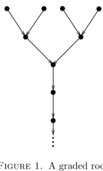
Figure 1. A graded root
Next we turn to the case when exactly one ofpandqis even. The proof in this case requires some preparation from lattice homology. (For a more thorough introduction to this subject see [21, 23].)
4.4. Lattice homology. In determining theι-complex associated to the double branched cover of a torus knot Tp,q, the concept of lattice homology will be extremally useful.
This theory was motivated by computational results of Ozsv´ath and Szab´o (for mani- folds given by negative definite plumbing trees of at most one ’bad’ vertex) in [27] and extended by N´emethi [21] to any negative definite plumbing trees. The isomorphism of lattice homology with Heegaard Floer homology was established for almost-rational graphs by N´emethi in [21], which was extended in [24] to graphs with at most two
’bad’vertices. Below we recall the basic concepts and results of this theory.
A graded root is a pair (R, w) where
• R is a directed, infinite tree with a finite number of leaves and a unique end modelled on the infinite stem • //• //• //· · ·, subject to the con- dition that every vertex has one and only one successor (see Figure 1 for an example),
• w: R → Q is a function associating to each vertex x of R a rational number w(x)∈Q such that w(x2) =w(x1)−2 if (x1, x2) is an edge of R.
A graded root (R, w) specifies a gradedF[U]-moduleH−(R, w) as follows: As a graded vector space,H−(R, w) is generated overFby the vertices ofR, graded so that gr(x) = w(x) for all x∈ R. Multiplication by U is defined on the set of generators by saying that U ·x=y if for the vertex x of R the vertex yis its successor.
Manolescu and Dai showed in [2] that the lattice homologyH−(R, wk) corresponding to the graded root (R, wk) can be represented as the homology of a model complex C(R), which is defined as follows. Let C(R) be generated (as an F[U]-module), by
• the leaves {vl} of R (with grading w(vl)), called the even generators, and
• by the odd generators defined as follows: for a vertex a of R with valency greater than 2, let V = {v1,· · · , vn} be the set of all vertices of R satisfying Uv =a. Then we take the formal sums v1−v2,· · · , vn−1−vn of vertices ofR as generators ofC(R) at degree w(a) + 1.
The U-action in this module lowers degree by 2. The differential ∂ on C(R) vanishes on all even generator v, while for an odd generator a the definition is slightly more complicated. Let v and w be two even generators such that a = Umv − Unw as
formal sums of vertices of R, for some nonnegative integersm andn. Then set∂(a) = Um+1v−Un+1w. In this case we say that the odd generatora is anangle between the even generators v and w. (For pictorial descriptions of C(R), see [2].)
A negative definite plumbing tree Γ (with associated plumbed four-manifoldXΓ) and a characteristic vectorkofH2(XΓ,Z) determines a graded root (RΓ, wk) as follows. Let L be the non-compact 1-dimensional CW-complex having the points of H2(XΓ,Z) = Z|Γ| as 0-cells and a 1-cell connecting two vertices ℓ, ℓ′ ∈ H2(XΓ;Z) if ℓ′ = ℓ+v for some v ∈ Γ. The characteristic vector k ∈H2(XΓ,Z) = Hom(H2(XΓ),Z) determines a quadratic function through the formula
χk(ℓ) =−1
2(k(ℓ) +ℓ2). (7)
For each n ∈ Z let Sn be the set of connected components of the subcomplex of L spanned by the vertices satisfyingχk ≤n. We defineRΓto be the graph with vertex set S
n≥0Sn, in which two verticesx1 and x2 are connected by a directed edge if and only if the elements x1 ∈ Sn and x2 ∈ Sn+1 (corresponding to components of the sublevel sets χk ≤n and χk≤n+ 1, respectively) satisfyx1 ⊂x2. We define wk: RΓ →Q for x∈Sn by the formula
wk(x) = k2+|Γ|
4 −2n.
A negative definite plumbing graph Γ is rational if it is the resolution graph of a rational singularity, i.e. a singularity with geometric genuspg = 0. Note that according to [22, Theorem 1.3] a negative definite graph is rational if and only if the boundary YΓ of the associated four-dimensional plumbing XΓ is a Heegaard Floer L-space. We say that Γ is almost-rational if there is a vertex v of Γ on which we can change the weight in such a way that the result is rational.
Theorem 4.3. ([27]) Let Γ be an almost-rational graph, s∈Spinc(YΓ) a spinc struc- ture on YΓ, and k a characteristic vector of the intersection lattice of XΓ representing a spinc structure that restricts to s on the boundary ∂XΓ = YΓ. Then there is an isomorphism H−(RΓ, wk)≃HF−(YΓ,s) of graded F[U]-modules.
4.5. Torus knots again. With this preparation in place, we now return to the com- putation of invariants of torus knots. We start by describing a plumbing presentation of Σ(Tp,q), where the covering involutionτ is also visible.
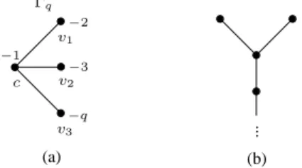
Lemma 4.4. Suppose that (p, q) = 1 and pq even. The plumbing graph Γ = Γp,q
presenting the double branched cover Σ(Tp,q) of S3 branched alongTp,q can be assumed to have the following properties:
• Γ is star-shaped with three legsLf ix, L1, L2 going out from the central vertex c.
• The coefficients on L1 and L2 are the same.
• The covering involution on Σ(Tp,q) can be modelled by a map on Γ which fixes Lf ix and c, and flips L1 and L2.
• The covering involution on Σ(K) extends smoothly to the plumbed 4-manifold XΓ, which is compatible with the above involution on Γ.
Proof. Recall that the double branched cover Σ(Tp,q) is equal to the link of the hy- persurface singularity z2 = xp +yq, hence Σ(Tp,q) can be presented as a plumbed manifold along the resolution dual graph of the above singularity. This graph can be easily determined by computing first the embedded resolution of the curve singu- larity xp +yq = 0, and then using a simple algorithm (described, for example in [5, Section 7.2]) for computing the resolution graph of the singularity. The embedded
resolution of Tp,q gives a linear graph, where the single (−1)-curve is intersected by the proper transform of the knot, and the multiplicities at the two ends are p and q, respectively (see [3]). Now [5, Lemma 7.2.8] shows that if say p is even, then the curves between the leaf with multiplicitypand the (−1)-curve intersecting the proper transform have all even multiplicities. The algorithm described in [5, Section 7.2]
then provides the resolution graph, together with the information about the covering transformation, satisfying the properties listed in the lemma.
Lemma 4.5. Suppose that Γ is a plumbing graph as in Lemma 4.4 and the action of τ exchanges the two legs. Then the associated reduced connected homology vanishes.
Proof. This information will be sufficient to identify the Z/2Z-action on the associ- ated graded root R. Recall that in computing a graded root, we have to choose a characteristic vector k ∈ H2(XΓ;Z), so that we can work with the induced weight function χk. Here, we choose k to be the canonical characteristic vector, which is given by k(v) = −2 −v2, where v2 denotes the self-intersection of the vertex v in the plumbing graph. Then k is clearly Z/2Z-invariant, so the induced spinc struc- ture [k]|∂WΓ ∈ Spinc(Σ(K)) on the boundary is also Z/2Z-invariant. Recall that the Z/2Z-action on the set of spinc structures on Σ(K) leaves the unique spin structure s0 invariant. Actually, even more is true: s0 is the unique fixed point of the action, as shown in [7, Page 1378] and [16, Remark 3.4]. Hence the lattice homology of Γ with respect tok computes HF−(Σ(K),s0). Since we are using aZ/2Z-invariant char- acteristic vector, the associated graded root Rk, computed using the weight function χk, admits aZ/2Z-action which acts by permuting its vertices. In conclusion, Rk is a symmetric graded root (in the terminology of [2, Definition 2.11]).
Next, we claim that there exists a Z/2Z-invariant vertex v ∈ V(Rk) with minimal χk-value. To prove this, we have to find a lattice point x = P
xv ·v ∈ Z|Γ| which satisfies the following properties:
• xisZ/2Z-invariant, i.e. the coefficients ofxon the arm L1 and the coefficients of x onL2 are the same.
• χk(x)≤χk(y) for any other lattice point y=P
v∈V(Γ)yv·v.
Once we have found such a lattice points, the claim about the vertex v can be proved using the following argument. Recall that vertices of Rk are components of sublevel sets ofχk. TheZ/2Z-action onRk permutes the components of sublevel sets, hence if we denote the component of the minimally-weighted sublevel set which contains the invariant lattice point x by C, then C is fixed by theZ/2Z-action.
To see the existence ofxwith the above properties, we first choose any lattice point x0 =P
v∈V(Γ(x0)v ·v such thatχk(x0) is minimal. Then we can write χk(x0) as χk(x0) =χk(xf ix0 ) +Q1(x0) +Q2(x0),
where xf ix0 = P
v∈Lf ix∪cxv ·v is the ”fixed part” x0 and Q1, Q2 are functions defined onZ|Γ| using the formula
−2Qi(x) = X
v∈Li
(x2v·ev +xvkv) + X
edge (v1v2) inLi
xv1xv2 +xvcixc
fori= 1,2. (Here, we have denoted the vertex in Li which is connected to the central vertex c asvic.)
Assume, without loss of generality, that Q1(x0) ≤ Q2(x0), and consider the lattice point x′ defined as
x′ =xf ix0 + X
v∈V(L1)
xv·(v+σ(v)), where σ denotes the Z/2Z-action on Γ. Then we have
χk(x′) =χk(xf ix0 ) + 2Q1(x0)≤ χk(x0) +Q1(x0) +Q2(x0) =χk(x0).
Since we assumed that χk(x0) is minimal among all lattice points, we get χk(x′) = χk(x0), implying x′ satisfies the desired properties.
Now we claim that our symmetric graded root R = Rk is locally equivalent to another symmetric graded root R′, where the Z/2Z-action on R′ is trivial. This can be verified by induction on the number nR of non-Z/2Z-invariant leaves ofR. In this part of the proof, in the notation we will confuse graded roots with their associated model complexes. For example, when we write that two given symmetric graded roots are locally equvialent, we will actually mean that their associated model chain complexes are locally equivalent.
The base case is simple: if nR = 0, then the Z/2Z-action on R is already trivial, so we are done. In the general case, choose a non-Z/2Z-invariant leaf v of R. Since R carries a Z/2Z-invariant leaf in its top-degree level, we can always find a Z/2Z- invariant vertex x of R which lies in the same grading as v does. Denote the angle between the infinite monotone path starting at v and at x by α. Then we define R1
as the graded root associated to the model complex we get from the model complex of R by deleting v, σ(v) and the angles α, σ(α). Define a map F from the associated model complex of R to that of R1 as follows.
• F(v) =F(σ(v)) =x and F(w) = wfor any leaf w6=v.
• F(α) =F(σ(α)) = 0 and F(β) =β for any angle β 6=α.
• Extend this mapF[U]-linearly to the model chain complex of R.
This mapF is obviously F[U]-linear and Z/2Z-equivariant, so if we only prove thatF is a chain map, it would automatically be a local equivalence to its image. To check thatF is a chain map, it suffices to check that∂(F(v)) =F(∂v) and∂(F(α)) =F(∂α) by linearity and equivariance. Indeed,
• ∂(F(v)) = ∂(even generator) = 0 andF(∂v) = F(0) = 0,
• ∂(F(α)) =∂(0) = 0 and F(∂α) =F(v+x) =F(v) +F(x) =x+x= 0.
Consequetly F is a local equivalence. This implies thatR is locally equivalent toR1, and the number of non-Z/2/Z-invariant leaves ofR1 is strictly smaller than the number of non-Z/2Z-invariant leaves of R. Thus, by induction, we deduce that R is locally equivalent to a symmetric graded root R′ whose Z/2Z-action is trivial. This gives us the equality δ(K) =δ(K), which by Proposition 3.7 then implies the claim.
Proof of Theorem 1.5. Proposition 4.2 in the case pq odd, and the combination of Lemmas 4.4 and 4.5 show that the covering transformation on Σ(Tp,q) is homotopic to id. The rest of the statement then follows as for the case of alternating knots.
5. Arborescent and Montesinos knots
A plumbing tree Γ is a tree whose vertices are labelled by integers (see Γ on Figure 2 below). Above we associated a four-manifoldXΓ(and its three-dimensional boundary YΓ) to a plumbing tree Γ. A variant of this construction associates a surface FΓ ⊂S3 to Γ: for every vertex we consider an annulus or a M¨obius band, given by introducing
00 11
00 11 00
11 000111 000000000 000000000 000000000 000000000 000000000 111111111 111111111 111111111 111111111 111111111
000000000 000000000 000000000 000000000 000000000 111111111 111111111 111111111 111111111 1111111110000000011111111 0
−2
3
−1
FΓ
Γ KΓ
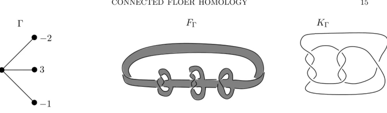
Figure 2. The plumbing graph Γ on the left determines a surfaceFΓ (shown in the middle) with boundaryKΓ.
half-twists dictated by the label of the vertex, and plumb (or Murasugi sum) these annuli and M¨obius bands together according to Γ. (See Figure 2 for a simple example.) The boundary ofFΓ specifies a linkKΓ =∂FΓ, called anarborescent link associated to Γ.
Remark 5.1. Notice that the link is not determined uniquely by the graph, since at vertices of higher valency we need to determine an order for the edges when considering a planar presentation, and the link might depend on this choice. In addition, the location of the plumbing region relative to the twists also might influence the resulting link. With slightly more information (see Gabai’s introductory work in [4]) attached to the tree this procedure can be made unique, though.
The resulting KΓ is called aMontesinos link if the tree Γ is star-shaped (i.e., has at most one vertex with valency more than 2); it is apretzel link if Γ is star-shaped with all legs of length one, and is 2-bridge if Γ is linear (i.e., all valencies are either 1 or 2).
The construction of the four-manifold and the knot associated to Γ is connected by the fact that (by repeated application of Montesinos’ trick) the double branched cover Σ(KΓ) of an arborescent link KΓ is homeomorphic to the boundary YΓ of the four-dimensional plumbing XΓ associated to Γ. Indeed, XΓ can be presented as the double branched cover ofD4 branched along the surface we get by pushing the interior of the surfaceFΓ of the above pluming into D4.
Next we give an algorithm for computing the connected Floer homology group HFB−conn(K) of an arborescent knot based on lattice homology. Recall that the graded module H−(R, w) associated to a graded root (R, w) is the homology of a canonical free, finitely generated chain complex (the model complex) (C(R), ∂) over the polyno- mial ring F[U]. The following was observed in [2, Remark 4.3].
Lemma 5.2. If (R, w) is a graded root, then a grading preserving homomorphism f: H−(R, w)→H−(R, w)lifts, uniquely up to chain homotopy, to a grading preserving chain map f#: C(R)→C(R). In addition, ifC is a free chain complex with H∗(C)≃
H−(R, w) then C ≃C(R).
Ifk is a characteristic vector which restricts to a self-conjugate spinc structure s0 ∈ Spinc(YΓ), then the graded root (RΓ, wk) comes with an involution J: H−(R, w) → H−(R, w) [2, Section 2.3]. This is the map induced on H−(R, w) by
ℓ 7→ −ℓ− 1
2P D(k), (8)
for ℓ∈H2(XΓ,Z). We denote its lift to C(R) by J#: C(RΓ)→C(RΓ).
Theorem 5.3. Let K = KΓ be an arborescent knot associated to an almost-rational plumbing treeΓ. Then there exists a chain homotopy equivalence(CF−(Σ(K),s0), τ#)≃ (C(RΓ), J#) of ι-complexes.
Proof. Letk0 ∈ H2(XΓ,Z) be a characteristic vector of the intersection lattice of XΓ
which restricts tos0 on the boundary. Theorem 4.3 provides an isomorphism H∗(CF−(Σ(K),s0)) = HF−(Σ(K),s0)≃H−(RΓ, wk0) =H∗(C(RΓ)) .
As a consequence of Lemma 5.2, if we prove that the push-forward ofJ: H−(RΓ, wk0)→ H−(RΓ, wk) through this isomorphism agrees withτ∗: HF−(Σ(K),s0)→HF−(Σ(K),s0), we are done.
Denote by WΓ the cobordism S3 →YΓ obtained from XΓ by removing the interior of a small ballD4 ⊂XΓ. Unravelling the definition of the isomorphism of Theorem 4.3 as it was done in [11, Theorem 3.1], the claim boils down to the identity
τ#◦FW−Γ,k =FW−Γ,−k ,
where k is a characteristic vector which restricts to s0 on the boundary. According to [36] the covering involution τ: YΓ → YΓ extends over XΓ to the complex conjugation T: XΓ →XΓ. SinceT acts on spincstructures as spinc conjugation, Lemma 3.6 implies
the claimed identity.
By applying similar arguments of [2, Section 5] we get the following results.
Corollary 5.4. Let K = KΓ be an arborescent knot associated to an almost-rational plumbing tree Γ. Then there is an isomorphism of graded F[U]-modules HFB−(K) ≃ Ker (1+J)[−1]⊕CoKer (1+J). Under this isomorphism the action ofQonHFB−(K) is given by the projection Ker (1 +J)→Ker (1 +J)/Im(1 +J)⊂CoKer (1 +J).
Corollary 5.5. Let K = KΓ be an arborescent knot associated to an almost-rational plumbing tree Γ. Then δ(K) =δ(K) and δ(K) = −σ(K)/4, where σ(K) denotes the signature of K.
Proof. Following the argument of [11, Theorem 1.2] we can identify δ(K) with the Ozsv´ath-Szab´o correction term of the double branched cover d(Σ(K),s0) = δ(K).
Furthermore, δ(K) = −2·µ(Γ,s0) where µ(Γ,s0) denotes the Neumann-Siebenmann µ-invariant of the plumbing Γ in the spin structure s0. On the other hand, according to [35, Theorem 5] we have σ(K) = 8·µ(Γ,s0) thus δ(K) =−σ(K)/4.
Note that since a star-shaped plumbing tree Γ is almost-rational, for Montesinos knots the assumption of the above results modifies to demand that the intersection form of XΓ (equivalently, the inertia matrix of the plumbing graph Γ) is negative definite. This method of approaching computability questions will be utilized in the next section.
The connected group associated to theι-complex (C(R), J#) of a graded root (R, w) can be easily computed. Given a vertex v ∈R denote by C(v) the set of all leaves of R that are connected to v by an oriented path. We construct a subset S of the leaves of R by the following algorithm. Let v0 denote the J-invariant vertex v0 of R with highest weight. If C(v0) consists of only one vertex, we add it to S; otherwise, we can find a pair{v, Jv}inC(v0) and in this case we add bothv andJvtoS. Next consider the path γ connecting v0 to infinity. Take v1 ∈ R to be the first vertex along γ for which C(v0) ( C(v1). If C(v1) contains a pair of leaves {v, Jv} with weight larger than the weight of any leaf in S then we choose one such pair with largest possible weight and we add it to S. By keep iterating this procedure until γ merges with the