arXiv:2010.04967v1 [math.GT] 10 Oct 2020
ANDR ´AS I. STIPSICZ AND ZOLT ´AN SZAB ´O
Abstract. We introduce a numerical invariantβ(K)∈N of a knot K⊂S3 which measures how non-alternating K is. We prove an inequality between β(K) and the (knot Floer) thickness th(K) of a knot K. As an application we show that all Montesinos knots have thickness at most one.
1. Introduction
A knot K⊂S3 isalternating if it admits a diagram with the property that when traversing through the diagram, we alternate between over- and under-crossings.
(An intrinsic definition of alternating knots have been recently found by Greene and Howie [4, 5].) A diagram of K partitions the plane into domains (the connected components of the complemet of the projection), and the alternating property can be rephrased by saying that on the boundary of each domain each edge connects an under-crossing with an over-crossing. Indeed, this observation provides a way to measure how far a knot is from being alternating. We introduce the following definition:
Definition 1.1. Suppose that D is the diagram of a given knot K ⊂ S3. A domain d of D isgood if any edge on the boundary of d connects an over- and an undercrossing. The domain d isbad if it is not good. The number of bad domains of the diagram D is denoted by B(D).
Obviously the diagram D is alternating iff B(D) = 0 . Indeed, by taking β(K) = min{B(D)|D diagram for K}
we get a knot invariant, which satisfies that β(K) = 0 if and only if K is an alternating knot. As it is typical for knot invariants given by minima of quantites over all diagrams, it is easy to find an upper bound onβ(K) (by determining B(D) for a diagram of K), but it is harder to actually compute its value.
As it turns out, knot Floer homology provides a lower bound for β(K) through the thickness of K. Recall that HFK(K), the hat-version of knot Floer homology of[ K is a finite dimensional bigraded vector space over the field F of two elements. By collapsing the Maslov and Alexander gradingsM andAon HFK(K) to[ δ=A−M we get a graded vector space HFK[δ(K). The thickness th(K) of K is the largest possible difference of δ-gradings of two homogeneous (nonzero) elements of this vector space. It is known that for an alternating knot K the δ-graded Floer homology is in a single δ-grading (determined by the signature of the knot), hence if K is alternating, then th(K) = 0 . (Knots satisfying th(K) = 0 are calledthin knots, hence alternating knots are thin.)
1
With this definition in place, the main result of this paper is
Theorem 1.2. Suppose that K⊂S3 is a non-alternating knot. Then
(1.1) th(K)≤ 1
2β(K)−1.
While the thickness of K can be used to estimate how non-alternating K is, the formula of Equation (1.1) also can be used to estimateth(K) by finding appropriate diagrams of K. In particular, the formula can be applied to show
Corollary 1.3. (Lowrance [6]) Suppose that K is a Montesinos knot. Then, th(K)≤1.
Remark 1.4. A quantity similar to β(K) has been introduced by Turaev[8], now called theTuraev genus gT(K). An inequality similar to Inequality (1.1)for the Turaev genus and the (knot Floer) thickness th(K) was shown by Lowrence in [6].
As the Turaev genus of non-alternating Montesinos knots is known to be equal to 1[1, 2], our Corollary 1.3 also follows from [6].
The formula of Inequality (1.1) can be used in a further way: by a recent result of Zibrowius [9] mutation does not change HFK[δ(K), hence leavesth(K) unchanged.
Consequently, besides isotopies we can change a diagram by mutations to get better estimates for th(K) through B(D) for a diagram D of a mutant.
The paper is organized as follows. In Section 2 we recall basics of knot Floer homology and prove the theorem stated above. In Section 3 we give the details of the proof of Corollary 1.3, and finally in Section 4 we list some further properties and questions regarding β.
Acknowledgements: AS was partially supported by theElvonal (Frontier) project´ of the NKFIH (KKP126683). ZSz was partially supported by NSF Grants DMS- 1606571 and DMS-1904628. We would like to thank Jen Hom and Tye Lidman for a motivating discussion.
2. The knot Floer homology thickness of knots Suppose thatV =P
aVa is a finite dimensional graded vector space, whereVa⊂V is the subspace of homogeneous elements of grading a∈R. The thickness th(V) of V is by definition the largest possible difference between gradings of (non-zero) homogeneous elements:
th(V) = max{a∈R|Va6= 0} −min{a∈R|Va6= 0}.
Suppose now that the graded vector space V is endowed with a boundary operator
∂ of degree 1 ; then the homology H(V, ∂) also admits a natural grading from the grading of V. As H(V, ∂) is the quotient of a subspace of V, it is easy to see that
th(H(V, ∂))≤th(V).
The hat version of knot Floer homology (over the field F of two elements) of a knot K⊂S3is a finite dimensional bigraded vector spaceHFK(K) =[ P
M,AHFK[M(K, A).
0 0
−1/2
1/2
0 0 0 1
0 0
0
−1 M:
0 0
−1/2
−1/2
0 0
1/2
1/2 δ:
0 0
1/2
−1/2 A:
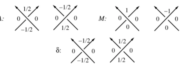
Figure 1. The local contributions for A, M and δ at a crossing. The Kauffman state distinguishes a corner at the cross- ing, and we take the value in that corner as a contribution of the crossing to A, M or δ of the Kauffman state at hand.
By collapsing the two gradings to δ = A−M, we get the δ-graded invariant HFK[δ(K). The thickness of HFK[δ(K) is by definition the thickness th(K) of K. Knot Floer homology is defined as the homology of a chain complex we can associate to a diagram of the knot (and some further choices). Indeed, for a given diagramD of a knot K fix a marking, that is a point of D which is not a crossing. Consider the bigraded vector space CD,p (graded by the Alexander and the Maslov gradings A and M) associated to the marked diagram (D, p), which is generated overF by the Kauffman states of the marked diagram, a concept which we recall below.
Suppose that for the marked diagram (D, p) of the knot K the set of crossings is denoted by Cr(D), the set of domains by Dom(D), andDomp(D) denotes the set of those domains which do not containpon their boundary. AKauffman state κis a bijectionκ: Cr(D)→Domp(D) with the property that for a crossingc∈Cr(D) the value κ(c) is one of the (at most four) domains meeting at c. The Alexander, Maslov and δ-gradings of a Kauffman state are computed by summing the local contributions at each crossing, as given by the diagrams of Figure 1.
According to [7] there is a boundary map ∂:CD,p→CD,p of bidegree (−1,0) (in the bigrading (M, A)) with the property that H(CD,p, ∂) =HFK(K) is isomorphic[ to the knot Floer homology of K (as a bigraded vector space). By collapsing the two gradings A and M to δ=A−M, we get the graded vector spaces (CD,pδ , ∂) and its homology HFK[δ(K). As HFK[δ(K) is the quotient of a subspace of CD,Pδ , we have that th(HFK[δ(K))≤th(CD,pδ , ∂).
Proposition 2.1. Suppose that D is a diagram of the knot K. If D is not an alternating diagram, then
th(CD,pδ )≤1
2B(D)−1.
Proof. Fix a marked point p on D, and consider the δ-graded chain complex (CD,pδ , ∂) generated by the Kauffman states of (D, p).
The δ-grading at a positive crossing is either 0 or −12, and at a negative crossing it is either 0 or 12. So we can express the δ-grading of a Kauffman state κ as the sum
−1
4wr(D) + X
c∈Cr
f(κ(c)),
. . . .
1
2 3 4 5
6
7
r
r r r r
r r
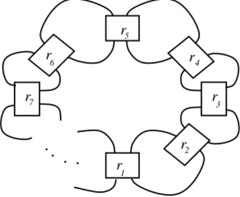
Figure 2. The Montesinos knot M(r1, . . . , rn). The box con- taining ri denotes the algebraic tangle determined by the rational number ri = αβii (cf. Figure 3). In order to have a knot, at most one of αi can be even.
where wr is the writhe of the diagram, andf is a function on the Kauffman corners, which is either 14 or −14 (depending on the chosen quadrant at the crossing c).
Simple computation shows that for a good domain each corner in the domain gives the same f-value, hence for different Kauffman states the contributions from this particular domain are the same. This is no longer true for a bad domain, but the difference of two contributions is at most 12. When determining the possible maxi- mum of δ(x)−δ(x′) for two homogeneous elements x, x′∈CD,pδ , the contributions from the writhe cancel, and so do the contributions from good domains, while bad domains contribute at most 12. This shows that th(CD,pδ )≤ 12B(D).
By assumption D is not alternating, hence there is a bad domain, with an edge showing that it is bad. Choose the marking p on such an edge. Since this edge guarantees that the two domains having it on their boundary are both bad, while these two bad domains do not get Kauffman corners, we get that th(CD,p) is bounded by 12(B(D)−2) = 12B(D)−1 , concluding the proof.
Proof of Theorem 1.2. Suppose that K is not alternating. Then any diagram D of K is non-alternating, hence we have that
th(K)≤th(CD,pδ )≤1
2B(D)−1.
Sinceβ(K) is computed from the minimum of the right-hand side of this inequality,
the proof follows at once.
3. Montesinos knots
Montesinos knots are straighforward generalizations of pretzel knots; a diagram involving rational tangles defining the Montesinos knot M(r1, . . . , rn) is shown by Figure 2. (A box with a rational number ri in it symbolizes the tangle shown by Figure 3.) We allow any of the ri to be equal to ±1 . Notice that the order of (r1, . . . , rn) is important; those ri which are equal to ±1 can be commuted with any other parameter through a simple isotopy of the diagram.
.. .
.. .
r c
c
c c
1
2
n n
Figure 3. The rational tangle corresponding tor∈Q. Here the boxes with ci ∈ Z on the right denote |ci| half twists (right handed for positive, left handed for negativeci). Depending on the parity ofn(the numbre ofci) we have two different finishing forms.
The rational number r determines the coefficients ci through its continued fraction expansion. The tangle is alternating (as part of a knot or link) if ci alternate in signs.
c c
c c
2 −2
1 1 1 1
2
2 1
1
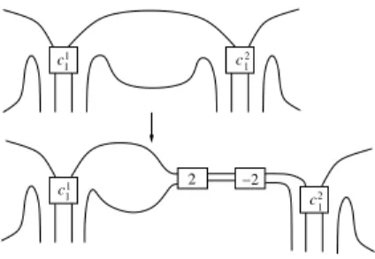
Figure 4. The introduction of cancelling twists to turn domains between tangles good.
Lemma 3.1. Consider the diagram of the Montesinos knot M(r1, . . . , rn) given by Figure 2. It can be isotoped to a diagram with at most four bad domains.
Proof. Recall that a rational tangle has the form given by Figure 3. Adapting the isotopies described in [3], we can achieve that all tangles are alternating, hence the potentially bad domains are the ones between the tangles, together with the central and the unbounded domains. The number of bad domains between the tangles can be reduced by the following observation. The domain between two tangles is bad if the first coefficients c11 and c21 of the two rational numbers determining the tangles have opposite signs, say c11>0 and c21<0 . Then by Reidemestier-II moves we can introduce cancelling twistings, as shown by Figure 4, and then commute the first twisting (in the figure given by the box with 2 in it) between the first and second tangles of the Montesinos knot. All domains between the boxes will become good, except the ones connecting the first tangle with the newly introduced twists and the second tangle also connecting it with the newly introduced twists. After these alterations make sure that (by the adaptation of [3]) all tangles are isotoped to be alternating. In total the new diagram then has four bad domains, concluding the
proof.
Proof of Corollary 1.3. For a Montesinos knot M(r1, . . . , rn) an approrpiate iso- topy of the diagram of Figure 2 (as given by Lemma 3.1) gives a diagram with at most four bad domains. The application of Theorem 1.2 concludes the argu-
ment.
Remark 3.2. Using the mutation invariance of th(K), Lemma 3.1 can be avoided:
by mutations any Montesinos knot M(r1, . . . , rn) can be moved to M(q1, . . . , qn) with the same rational parameters in a different order so that qi and qi+1 have the same sign with at most one exception. Isotoping the diagram so that the tangles are alternating, the mutated diagram then has at most 4 diagrams. Using the result of [9]then the corollary follows as before.
4. Further properties
It is a standard fact that the knot Floer homology of the connected sum of two knots is the tensor product of the knot Floer homologies:
HFK(K[ 1#K2)∼=HFK(K[ 1)⊗HFK(K[ 2).
From this (bigraded) isomorphism it follows that
th(K1#K2) =th(K1) +th(K2).
The behaviour of β(K) is less clear under connected summing. Suppose that K1, K2 are both non-alternating knots. By taking the connected sum of two di- agrams D1, D2 for these knots at bad edges (i.e. arcs on the boundary of bad domains verifying that the domains are bad) we get that
B(D1#D2) =B(D1) +B(D2)−2, immediately implying that
β(K1#K2)≤β(K1) +β(K2)−2.
Motivated by the equality for the thickness th, we conjecture Conjecture 4.1. If K1, K2 are two non-alternating knots, then
β(K1#K2) =β(K1) +β(K2)−2.
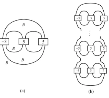
It is not hard to find knot diagrams for which Inequality (1.1) is sharp. Indeed, the standard diagram of the pretzel knot P(−3,5,5) admits four bad domains (see Figure 5(a)), while an explicite calculation of HFK(P[ (−3,5,5)) shows that th(P(−3,5,5)) = 1 . Consider the n-fold connected sum Kn = #nP(−3,5,5);
connect summing the diagrams at bad edges (in the above sense) we get a sequence of knots Kn and diagramsDn for them with the properties that th(Kn) =n and B(Dn) = 2n+ 2 , cf. Figure 5(b). The non-alternating knots Kn then satisfy n=th(Kn) =12β(Kn)−1 .
−3 5 5
−3 5 5
−3 5 5
...
5 5
−3
B B
B B
(a) (b)
Figure 5. In (a) he pretzel knot P(−3, ,5,5) is shown. The B symbols signify the bad domains. (A box containing the integer n denotes |n| half twists, right handed forn >0 and left handed for n <0 .) In (b) we provide a diagram of Kn, where the connected sum is taken at bad domains.
References
[1] A. Champanerkar and I. Kofman. A survey on the Turaev genus of knots.Acta Math. Viet- nam., 39(4):497–514, 2014.
[2] O. Dasbach, D. Futer, E. Kalfagianni, X.-S. Lin, and N. Stoltzfus. The Jones polynomial and graphs on surfaces.J. Combin. Theory Ser. B, 98(2):384–399, 2008.
[3] J. Goldman and L. Kauffman. Rational tangles.Adv. in Appl. Math., 18(3):300–332, 1997.
[4] J. Greene. Alternating links and definite surfaces.Duke Math. J., 166(11):2133–2151, 2017.
With an appendix by Andr´as Juh´asz and Marc Lackenby.
[5] J. Howie. A characterisation of alternating knot exteriors.Geom. Topol., 21(4):2353–2371, 2017.
[6] A. Lowrance. On knot Floer width and Turaev genus.Algebr. Geom. Topol., 8(2):1141–1162, 2008.
[7] P. Ozsv´ath and Z. Szab´o. Heegaard Floer homology and alternating knots. Geom. Topol., 7:225–254, 2003.
[8] V. Turaev. A simple proof of the Murasugi and Kauffman theorems on alternating links.
Enseign. Math. (2), 33(3-4):203–225, 1987.
[9] C. Zibrowius. On symmetries of peculiar modules; or, δ-graded link Floer homology is muta- tion invariant. arXiv:1909.04267, 2019.
R´enyi Institute of Mathematics, H-1053 Budapest, Re´altanoda utca 13–15, Hungary Email address:stipsicz.andras@renyi.hu
Department of Mathematics, Princeton University, Princeton, NJ, 08544 Email address:szabo@math.princeton.edu