One-loop constituent quark contributions to the vector and axial-vector meson curvature mass

curvature mass

Gy˝oz˝o Kov´acs,^{1, 2,∗} P´eter Kov´acs,^{1, 2,†} and Zsolt Sz´ep^3,‡

1ELTE E¨otv¨os Lor´and University, Institute of Physics, P´azm´any P´eter s´et´any 1/A, 1117 Budapest, Hungary

2Institute for Particle and Nuclear Physics, Wigner Research Centre for Physics, Konkoly-Thege Mikl´os ´ut 29-33, 1121 Budapest, Hungary

3MTA-ELTE Theoretical Physics Research Group, P´azm´any P´eter s´et´any 1/A, 1117 Budapest, Hungary

The renormalized contribution of fermions to the curvature masses of vector and axial-vector mesons is derived with two different methods at leading order in the loop expansion applied to the (2 + 1)-flavor constituent quark-meson model. The corresponding contribution to the curvature masses of the scalar and pseudoscalar mesons, already known in the literature, is rederived in a transparent way. The temperature dependence of the curvature mass of various (axial-)vector modes obtained by decomposing the curvature mass tensor is investigated along with the (axial-)vector–

(pseudo)scalar mixing. All fermionic corrections are expressed as simple integrals that involve at finite temperature only the Fermi-Dirac distribution function modified by the Polyakov-loop degrees of freedom. The renormalization of the (axial-)vector curvature mass allows us to lift a redundancy in the original Lagrangian of the globally symmetric extended linear sigma model, in which terms already generated by the covariant derivative were reincluded with different coupling constants.

I. INTRODUCTION

The extension of the linear sigma model with vector and axial-vector degrees of freedom has a long history (see e.g. [1–3]). In recent years, much effort was in- vested in the study of the phenomenological applicability of various formulations of the model. It turned out, for example, that the gauged version of the model cannot re- produce the correct decay width of theρanda1 mesons [4], and therefore the interest shifted toward versions of the model which are based on the global chiral symmetry:

originally constructed for two flavors in [5] the extended linear sigma model (ELσM) was formulated for three fla- vors in [6].

The parametrization of the three-flavor ELσM in re- lation with hadron vacuum spectroscopy was thoroughly investigated in [6]. Constituent quarks were incorporated in the ELσM in [7] and their effect on the parametriza- tion, through the correction induced in the curvature masses of the scalar and pseudoscalar mesons, was in- vestigated along with the chiral phase transition at fi- nite temperature and density. It is interesting to know how the model parameters and the results obtained in [7]

are influenced by coupling the constituent quarks to the (axial-)vector mesons. The effect of the (axial-)vector mesons on the chiral transition was studied in [8] in the gauged version of the purely mesonic linear sigma model with chiralU(2)L×U(2)R symmetry, by using a rather crude approximation for the Lorentz tensor structure of the (axial-)vector curvature mass matrix, which was as-

∗kovacs.gyozo@wigner.hu

†kovacs.peter@wigner.hu

‡szepzs@achilles.elte.hu

sumed to have the vacuum form even at finite tempera- ture. Further investigations in the above-mentioned di- rections require the calculation of the mesonic and/or fermionic contribution to the (axial-)vector curvature mass matrix and its proper mode decomposition, as was done in many models dealing with the description of hot and/or dense nuclear matter [9–11]. Such a calculation within the linear sigma model would allow for a com- parison with in-medium properties of the (axial-)vector mesons obtained with functional renormalization group (FRG) techniques in [12–15].

The curvature masses of the scalar and pseudoscalar mesons were derived in the U(3)L×U(3)R symmetric constituent quark model in [16]. The method used there involved taking the second derivative with respect to the fluctuating bosonic field of the ideal gas formula for the partition function in which the quark masses depend on these bosonic fields. The result was subsequently used in a plethora of publications, even when it does not apply, as was the case of Ref. [17], which seem- ingly uses incorrectly the result of [16] to study the effect of the temperature and chemical potential on the vec- tor and axial-vector masses. The result derived in [16]

for (pseudo)scalar mesons cannot be directly applied for (axial-)vector mesons, simply because it is not enough to consider only the boson fluctuation-dependent fermion masses: due to their Lorentz index the momentum and (axial-)vector fields couple to form a Lorentz scalar in the fermion determinant resulting from the fermionic functional integral. Due to such terms, derivatives of the fermionic functional determinant with respect to the (axial-)vector fields give additional contributions, com- pared to the bosonic case.

Although the calculation of the leading order fermionic contribution to the (axial-)vector curvature mass matrix can be done by taking the second field derivative of the

arXiv:2105.12689v2 [hep-ph] 17 Sep 2021

functional determinant, it is much easier to take an equiv- alent approach and compute the self-energy at vanishing momentum with standard Feynman rules. The techni- cal issues that need to be addressed are the mode de- composition and renormalization of the self-energy and the mixing between the (axial-)vector and (pseudo)scalar mesons.

We also mention that while our focus here is on the curvature mass, the pole mass and screening mass can also be obtained from the analytic expression of the self- energy calculated at nonzero momentum using the usual definitions given in Eq. (6) of [18], where the relation between the pole and curvature masses of the mesons was investigated with FRG techniques within the two- flavor quark-meson model. This difference depends on the approximation used to solve the O(N) and quark- meson models and it is typically larger for the sigma than the pion [18–21].

The organization of the paper is as follows. In Sec. II an approximation scheme is presented for a consistent computation of the effective potential (pressure) in the ELσM which is based on curvature masses that include the fermionic correction at one-loop level. In Sec. III we compute in the one-flavor case, Nf = 1, the cur- vature mass matrix of the mesons, with both methods mentioned above. This allows for the introduction of the relevant integrals used also in Sec. IV, where the self-energy of all the mesons is calculated at vanishing momentum for Nf = 2 + 1 flavors. In this case a di- rect calculation of the curvature masses from the func- tional determinant, although completely straightforward, is made cumbersome by the large number of fields and the dimension of the matrix involved. This calculation is relegated to Appendix D. Based on the mode decompo- sition of the (axial-)vector self-energy, presented in de- tail in Appendix E, the curvature masses of the phys- ical modes are given in terms of simple integrals. We also show in Sec. IV how to connect the expressions of the (pseudo)scalar curvature masses derived here with existing ones obtained with the alternative method of Ref. [16]. In Sec. V we discuss the renormalization of the (axial-)vector curvature masses in the isospin sym- metric case. Dimensional regularization was used in or- der to comply with the property of the vacuum vec- tor self-energy observed for some flavor indices, which is related to current conservation, as discussed in Ap- pendix B. The renormalization process revealed that the Lagrangian of the ELσM can be written more ju- diciously compared to the form used in the literature, such that each term allowed by the chiral symmetry is included only once, in accordance with the gener- ally accepted procedure. By looking from a new per- spective at the wave-function renormalization factor re- lated to the (axial-)vector–(pseudo)scalar mixing, we dis- cuss in Sec. VI how the self-energy corrections modify its tree-level expression. Section VII contains numeri- cal results concerning the temperature evolution of the meson masses obtained in a new vacuum parametriza-

tion of the model which takes into account the one- loop fermionic correction in the curvature mass of all the mesons. Section VIII is devoted to conclusions and an outlook. The appendixes not mentioned here contain some further technical aspects used in the calculations.

II. LOCALIZED GAUSSIAN APPROXIMATION IN THE YUKAWA MODEL

In order to motivate our interest in the curvature mass, we present an improved calculational scheme for the ef- fective potential of the ELσM compared to that used in [7]. This scheme, which we call the localized Gaussian approximation, uses the curvature mass of the various mesons. To keep the notation simple, we consider the simplest chirally symmetric Yukawa model, defined by the Lagrangian

LY=1

2∂µϕ∂^µϕ−Ucl(ϕ) + ¯ψ i /∂−gSϕ)ψ, (1) where ψ and ϕ are fermionic and bosonic fields and U_cl(ϕ) =m²₀ϕ²/2 +λϕ⁴/24 is the classical potential. We use Minkowski metricg^µν = diag(1,−1,−1,−1) and the conventions of Ref. [22].

Integrating over the fermions in the partition function¹ Z =

Z

DϕDψDψe¯ ^iRxLY = Z

Dϕe^iA(ϕ), (2) leads to the action (R

x≡d⁴x) A(ϕ) =

Z

x

1

2∂µϕ∂^µϕ−Ucl(ϕ)

−iTr log iS⁻¹(∂;/ ϕ) , (3) where Tr≡trDR

d⁴xdenotes the functional trace, with the subscript “D” referring to the Dirac space, and

iS⁻¹(x, y) =

i /∂_x−gSϕ(x)

δ⁽⁴⁾(x−y) (4) is the inverse fermion propagator.

Shifting the field with an x-independent background φ, ϕ(x)→φ+ϕ(x), the effective potential can be con- structed along the lines of Ref. [23]. Several approxi- mations of the effective potential are considered in the literature.

a. Mean-field approximation The bosonic fluctuat- ing field is neglected altogether, leading to

UMF(φ) =Ucl(φ) +itrD

Z

K

log iS_f⁻¹(K) , (5) whereiS_f⁻¹(K) =K−m/ fis the tree-level fermion inverse propagator with massmf =gSφ. Here we introduced the notationR

K ≡R _d⁴_K

(2π)⁴ for the momentum integral with 4-momentum K^µ = (k0,k). The field equation used in [7] was derived in this approximation.

1In the LσM this step is motivated by the fact thatψrepresents the constituent quark, that is an effective degree of freedom not necessarily corrected by the interaction with mesons.

b. Ideal gas approximation The bosonic fluctuating field is neglected in the fermion determinant (Tr log) ap- pearing in Eq. (3) and kept only to quadratic order in the terms coming from the expansion ofU_cl(φ+ϕ). The Gaussian functional integral overϕleads to

U_eff^IG(φ) =UMF(φ)− i 2

Z

K

log iD⁻¹(K;φ) , (6) where iD⁻¹(K;φ) =K²−mˆ²(φ) is the tree-level boson propagator with ˆm²(φ) =d²Ucl(φ)/dφ² being the classi- cal curvature mass. This approximation was used in a nonsystematic way in [7] to include mesonic corrections in the pressure.

c. Ring resummation or Gaussian approximation The fermion determinant is expanded in powers ofϕand keeping in Eq. (3) the term quadratic in the fluctuat- ing mesonic field, the Gaussian functional integral over ϕresults in

U_eff^GA(φ) =U_MF(φ)−i 2

Z

K

log iD⁻¹(K;φ)−Π(K;φ) , (7) where the boson self-energy

Π(K;φ) =ig²_Str Z

P

S_f(P)S_f(K−P), (8) represents the one-loop contribution of the fermions. Ex- panding in Eq. (7) the logarithm one recognizes the in- tegrals of the ring resummation.

The ring resummation is widely used in the Nambu–

Jona-Lasinio model, where it goes by the name of random-phase approximation [24]. In that context the integral in Eq. (7) requires no renormalization and was evaluated using cutoff regularization in [25, 26]. To spare the trouble of renormalizing this integral in a lin- ear sigma model, one can approximate the self-energy with its zero momentum limit. In thislocalized approx- imation the dressed bosonic inverse propagator appear- ing in Eq. (7) is of tree-level type, just that the tree- level mass is replaced by the one-loop curvature mass Mˆ²(φ) ≡ mˆ²(φ) + Π(K = 0;φ). Since with a homo- geneous scalar background the curvature mass does not depend on the momentum, the renormalization of the in- tegral becomes an easy task, as discussed in [27] (see also Eq. (58) in Sec. V).

Note that one can define a curvature mass in each of the above approximations, by taking the second deriva- tive of the potential in Eq. (5), (6), or (7) with respect to the fieldφ.The curvature mass we investigate in this paper contains the fermionic contribution from the sec- ond field derivative of the Tr log in Eq. (3). This repre- sents the purely fermionic one-loop contribution to the curvature mass which can be derived in principle in the localized Gaussian approximation using the background field method.

In order to compute the pressure, we need to evaluate the effective potential at the minimum. In the localized

approximation the extremum, is determined as the solu- tion of the field equation

m²₀φ+λ 6φ³+1

2

λφ+ 2g_S³trD

Z

P

S_f³(P)

× Z

K

i

K²−Mˆ²(φ)−g_Str_D Z

K

Sf(K) = 0. (9) We mention that the second term in the square brackets is nothing but the fermionic correction to the three-point vertex function evaluated at vanishing momentum. This vertex function is obtained by expanding the fermionic determinant in powers of the bosonic field

Tr log iS_f⁻¹−gϕ

= Tr log iS_f⁻¹

−

∞

X

n=1

(−ig)ⁿ n

×trD

ⁿ Y

i=1

Z

d⁴xiϕ(xi)Sf(xi, xi+1)

xn+1=x1

. (10) The expansion gives a series of one-loop diagrams in which the nth term has n external fields (see e.g. [28]

or Ch. 9.5 of [22]). Using the background field method, the expansion of such a fermionic functional determinant was considered recently in [29, 30] in order to derive effec- tive couplings between constituent quarks, (axial-)vector mesons, and the photon.

The second field derivative of the functional determi- nant, taken at vanishing mesonic field, is nothing but the one-loop self-energy associated with the bosonic field with respect to which the derivative is taken, as the con- tribution of diagrams not having exactly two external fields of this type vanishes. Based on this observation one can obtain the lowest order fermionic correction to the bosonic curvature mass by computing the one-loop self-energy with standard Feynman rules.

III. CURVATURE MASS IN THENf = 1 CASE We generalize now Eq. (1) and consider the chirally symmetric Lagrangian²in which a fermionic fieldψinter- acts through a Yukawa term to scalar (S), pseudoscalar (P), vector (Vµ), and axial-vector (Aµ) fields

L_f = ¯ψ

iγ^µ∂_µ−g_S(S−iγ₅P)−g_Vγ^µ V_µ+γ₅A_µ ψ.

(11) The mesonic part of the Lagrangian is of the form L_m= X

X=S,P

h(∂X)² 2 −m²₀

2 X²i

− λ

4! S²+P²²

+ X

Y=V,A

h−1

4F_µν^Y F_Y^µν+m²_0,V 2 Y^µYµ

i

+L^int_m(X, Yµ),(12)

2The one-loop curvature mass formulas derived here can be easily modified when, in the absence of chiral symmetry,P andAcan have different Yukawa couplings thanSandV, respectively.

withF_µν^Y =∂µYν−∂νYµ.We shall return to the unspec- ified interacting part in theNf = 2 + 1 case in relation to the renormalization of the one-loop curvature masses.

By integrating over the fermions in the partition func- tion, done after the usual shifts S(x) → φ+S(x) (φ is independent of x) introduced in order to deal with the spontaneous symmetry breaking (SSB), one obtains a correction to the classical mesonic action in the form of a functional determinant. The expansion of the func- tional determinant in powers of mesonic field derivatives, the so-called derivative expansion [31, 32], leads to an effective bosonic action of the form

Z

d⁴xL_eff(φ, ξ) = Z

d⁴x

L_m(φ, ξ)−U_f(φ, ξ)+O((∂ξ)²) , (13) with the leading order term of the expansion being the one-loop fermionic effective potential

Uf(φ, ξ(x)) =iTr log iS_f⁻¹(∂;/ ξ)

=i Z

K

log detD iS_f⁻¹(K;ξ(x)) , (14) which depends on all the fluctuating mesonic fields col- lectively denoted byξ(x). We introduced

iS_f⁻¹(K;ξ) =K−m/ f−gS S−iγ5P

−gV V/+Aγ/ ₅), (15) for the inverse fermion propagator, in whichm_f =g_Sφ is the tree-level (classical) fermion mass. Hereafter thex dependence of the mesonic fields will not be indicated.

The second derivative of Uf(φ, ξ) with respect to the mesonic fields gives an additive correction to the classical mesonic curvature mass obtained from L_m. Since later we will investigate theN_f = 2 + 1 case, where the fields have flavor indicesa= 0, . . .8, we give the more general formulas of these corrections

∆ ˆm^2,(X)_ab ≡d²Uf(φ, ξ) dX_adX_b

_ξ=0

, X =S, P,

∆ ˆm^2,(Y_ab,µν⁾ ≡ −d²U_f(φ, ξ) dYa^µdY_b^ν

_ξ=0

, Y =V, A.

(16)

In this section the flavor indices should be disregarded.

The sign difference between the above definitions is due to the different signs of the corresponding clas- sical mass terms in Eq. (12). Accordingly, for the (pseudo)scalar field one has an additive correction to the classical mass squared ˆm^2,(X)_ab ≡ −_dX^d2Lm

adXb

_ξ=0, while for the (axial-)vector field the second derivative is a Lorentz tensor, and therefore the correction to

ˆ

m^2,(Y_ab ⁾≡ ^gνµ_{4 dY}^d2µ^Lm adY_b^ν

ξ=0depends on the tensor structure of ∆ ˆm^2,(Y_ab,µν⁾ and whether one works at zero or nonzero temperature. For example, at T = 0, where ∆ ˆm^2,(Y_ab,µν⁾ ∝ gµν, the fermionic correction to ˆm^2,(Y_ab ⁾ is obtained by taking the trace in Eq. (16):

∆ ˆm^2,(Y_ab ⁾:=1

4∆ ˆm^2,(Y_ab,µ^)µ. (17)

This is needed in a parametrization of the model that is based on the one-loop curvature masses. For the curva- ture mass at T 6= 0 one needs the mode decomposition of the tensor ∆ ˆm^2,(Yµν ⁾. This will be discussed in Sec. IV and Appendix E in relation to theN_f= 2 + 1 case.

A. Brute force calculation The determinant D≡det_D iS_f⁻¹(K;ξ)

appearing in Eq. (14) evaluates to

D=

g²_S (S+φ)²+P²

−K²² + K²−m²_f+g_V²V²−2gVK·V² +h

g²_VA²2

+ 2g_V²

(m²_f+K²)A²−2(K·A)²i + 2g_S²

(S+φ)²+P²−φ²

g²_V A²−V²

+ 2g_VK·V

− K²−m²_f²

. (18)

Writing the determinant in this form facilitates the derivation of the curvature masses, as the contribution to the scalar and the pseudoscalar comes only from the first term, while only the second and the third terms contribute in the case of the vector and the axial-vector, respectively. Also, note thatD(ξ= 0) = K²−m²_f²

. The second derivative of the determinant with respect to a particular field denoted byϕis calculated using

d²logD dϕdϕ

_ξ=0

= 1

D d²D dϕdϕ− 1

D² dD

dϕ dD

dϕ _ξ=0

. (19) Forϕ∈ {S, P, Vµ} this is applied writing D = ˜D²+R, where ˜D² is either the first or the second term on the right-hand side (rhs) of Eq. (18), while the remnant R does not contribute in Eq. (19). Introducing the notation Gf(K) = 1/(K²−m²_f) one obtains

d²logD dSdS

ξ=0

=−4g_S²

G_f+ 2m²_fG²_f

, (20a) d²logD

dP dP _ξ=0

=−4g_S²Gf, (20b) for the scalar and the pseudoscalar fields, and

d²logD dV^µdV^ν _ξ=0

= 4g²_V

gµνGf−2KµKνG²_f

, (21a) for the vector field.

For the axial-vector one applies Eq. (19) with D = D˜+R, where ˜D is the third term on the rhs of Eq. (18), to obtain

d²logD dA^µdA^ν _ξ=0

= 4g_V²

(m²_f+K²)gµν−2KµKν

G²_f.(21b) For scalar and vector fields there are contributions from both the first and the second derivative of ˜D, while in

the case of the pseudoscalar and axial-vector fields only the second derivative of ˜Dcontributes.

Using Eqs. (14), (16), (18), and (20) the fermion cor- rections to the curvature masses of the scalar and pseu- doscalar fields are obtained as

∆ ˆm^2,(S)=−4g_S²

1 + 2m²_f d dm²_f

T(mf), (22a)

∆ ˆm^2,(P)=−4g_S²T(mf), (22b) where the (vacuum) tadpole integral is

T(m_f) = Z

K

i K²−m²_f =

Z

K

iG_f(K). (23) In the case of the vector and the axial-vector fields, one evaluates the trace in Eq. (17), using Eqs. (16) and (21) together withg_µ^µ= 4 andKµKνg^νµ=K²=m²_f+G⁻¹_f , to obtain

∆ ˆm^2,(V)=−2g²_V

1−m²_f d dm²_f

T(mf), (24a)

∆ ˆm^2,(A)=−2g²_V

1 + 3m²_f d dm²_f

T(mf). (24b)

1. Integrals at finite temperature

The expressions in Eqs. (22) and (24a), which were formally derived at vanishing temperature (T = 0), can be easily generalized toT 6= 0, where the tadpole integral consists ofvacuum andmatter parts:

T(mf) =T⁽⁰⁾(mf) +T⁽¹⁾(mf). (25) The superscripts indicate the absence or the presence of statistical factors in the respective integrands. In a co- variant calculation the vacuum part T⁽⁰⁾(m_f) is the in- tegral in Eq. (23), while in a noncovariant calculation it is

T⁽⁰⁾(mf) =

Z d³k (2π)³

1

2(k²+m²_f)^1/2, (26) as obtained with the usual conventions of the imaginary time formalism [33], namely (µis the chemical potential)

k0→iνn+µ and Z

K

→iTX

n

Z d³k

(2π)³, (27) after doing the summation over the fermionic Matsubara frequenciesνn= (2n+ 1)πT. Thematter part is

T⁽¹⁾(m_f) =− 1 4π²

Z ∞

0

dk k² E_f(k)

f_f⁺(k) +f_f⁻(k) , (28) where f_f^±(k) = 1/(exp((E_f(k)∓µ)/T) + 1) are the Fermi-Dirac distribution functions for particles and an- tiparticles andE_f²(k) =k²+m²_f withk=|k|.

For the mass derivative of the matter part of the tad- pole integral (Euclidean bubble integral at vanishing mo- mentum) one usesd(f_f^±/Ef)/dm²_f =d(f_f^±/Ef)/dk² and an integration by parts to obtain

−B⁽¹⁾(mf)≡ dT⁽¹⁾(mf) dm²_f = 1

8π² Z ∞

0

dkf_f⁺(k) +f_f⁻(k) E_f(k) .

(29) The fact that even at finite temperature the trace of the second derivative appearing in Eq. (21a) is the only relevant quantity determining the curvature mass of the vector boson is due to current conservation. For the axial-vector this is not the case and one needs the mode decomposition of the tensor in Eq. (21b). This is dis- cussed in Appendix E.

B. Curvature mass from the self-energy As mentioned at the end of Sec. II, the one-loop cur- vature mass can also be obtained by computing the cor- responding zero momentum self-energy. For example, for the self-energy of the vector field, the Feynman rules ap- plied with the conventions of [22] give

iΠ^(V_µν⁾(Q= 0) =− −igV

2

trD

Z

K

γµSf(K)γνSf(K).

(30) UsingS_f =i(K/ +m_f)G_f, the Dirac trace

tr_D

γ_µ(K/ +m_f)γ_ν(K/ +m_f)

= 8K_µK_ν−4g_µνG⁻¹_f (K), (31) results in

Π^(V_µν⁾(Q= 0) =−4g_V²

gµνT(mf)−2i Z

K

KµKνG²_f(K)

. (32) Comparing Eq. (32) with the expression obtained by us- ing Eq. (21a) in Eq. (16) shows explicitly that ∆ ˆm^2,(Vµν ⁾= Π^(Vµν⁾(Q = 0). At zero temperature Π^(Vµν⁾(0) = 0 due to the current conservation related to theU(1)V global sym- metry, and therefore the one-loop curvature mass of the vector boson is the classical one, ˆm^2,(V).

In order to obtain the curvature mass of the physi- cal modes at finite temperature, we need the standard decomposition of the momentum-dependent self-energy tensor reviewed in Appendix E. The self-energy is decom- posed intovacuumandmatter parts. The former is eval- uated using a covariant calculation performed atT = 0 in a regularization scheme compatible with the consequence of current conservation, namely that the self-energy is 4- transverse, Q^µΠ^(Vµν⁾(Q) = 0, and Π^(Vµν,vac⁾ (Q = 0) = 0.

Therefore, only the matter part contributes to the self- energy components determining the curvature masses of the 3-longitudinal and 3-transverse vector modes

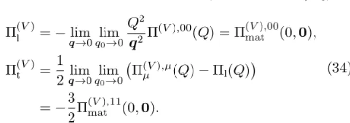
Mˆ_l/t^2,(V)= ˆm^2,(V)+ Π^(V_l/t⁾. (33)

The components are obtained as (see Ch. 1.8 of [34]) Π^(V_l ⁾=−lim

q→0 lim

q₀→0

Q²

q²Π^(V),00(Q) = Π^(V_mat^),00(0,0), Π^(V_t ⁾= 1

2 lim

q→0 lim

q0→0 Π^(V_µ ^),µ(Q)−Πl(Q)

=−3

2Π^(V_mat^),11(0,0).

(34)

For the axial-vector, which does not couple to a conserved current, the tensor structure of the self-energy is more complicated and it is discussed in Appendix E.

The interested reader can find in Appendix A a discus- sion on the matter part of the self-energy components.

For thevacuumpart see the discussion in Sec. V and the calculation presented in Appendix C.

IV. CURVATURE MASS FOR Nf = 2 + 1 The fermionic part of the chiral-invariant Lagrangian of the extended linear sigma model, whose mesonic part can be found in [7], has the form given in Eq. (11), only that the fermionic field is the triplet of constituent quarks, ψ ≡ (u, d, s)^T, while the mesonic fields are nonets. For the scalarsS=SaTa =Saλa/2,a= 0, . . . ,8 and similarly for the other mesons (λ_a6=0 are the Gell- Mann matrices andλ0=q

2 31).

The integration over the fermionic field in the partition function results in a functional determinant involving a N×N matrix, whereN= 3×4×N_cwithN_c being the number of colors. This matrix structure makes tedious a brute force calculation of the curvature mass similar to the one shown in Sec. III A, even in the case of a trivial color dependence (see Eq. (D1)). Therefore, we proceed as in Sec. III B by calculating the self-energy at vanishing momentum and relegate to Appendix D the sketch of a direct calculation.

A. Curvature mass from the self-energy For simplicity, we consider the case when only the scalar fields, namelyS0, S3andS8,have expectation val- ues, denoted by φ0, φ3, and φ8. It proves convenient to work in the N−S (nonstrange–strange) basis, which for a generic quantityQis related to the (0,8) basis by

QN

QS

=R Q0

Q8

, R=R⁻¹= 1

√3 √

2 1

1 −√ 2

. (35) Applying the above relation to the matrices λ0 and λ8, one obtainsλN= diag(1,1,0) andλS=√

2 diag(0,0,1), which give the antisymmetric structure constantsf_45N= f_67N = 1/2 and f_45S = f_67S = −1/√

2. With the shift Si → φi +Si, i = N,3,S, one obtains, using also λ3 = diag(1,−1,0), the tree-level inverse fermion propagator matrix in flavor space asiS¯₀⁻¹= diag(iS_u⁻¹, iS_d⁻¹, iS_s⁻¹),

TABLE I. Dirac matrices and couplings to be used in the self-energy formula (37).

X, cX,ΓX S,−igS,1 P,−gS, γ5 V,−igV, γµ A,−igV, γµγ5

with components iS_f⁻¹(K) = K/ −m_f, where the tree- level fermion masses are

mu,d=gS(φN±φ3)/2, ms=gSφS/√

2. (36)

The one-loop self-energy of a generic field Xa, witha being a flavor index, can be written as

Π^(X)_ab (Q) =iNcsXc²_X Z

K

trh ΓX

λa

2

S¯0(K)Γ⁰_Xλb

2 S¯0(L)i

, (37) where N_c is the number of colors, L= K−Q, s_X = 1 for X = V, A and sX = −1 for X = S, P. The prop- agator matrix ¯S0= diag(Su,Sd,Ss) has as elements the tree-level propagators of the constituent quarks. Further- more, ΓX contains Dirac matrices that carries a Lorentz index whenX ∈ {V, A}, in which case the prime on Γ⁰_X indicates that its Lorentz index is different from that of ΓX. The matrices are explicitly given in Table I, along with the constant cX proportional to the Yukawa cou- pling. The trace is to be taken in Dirac and flavor spaces.

We assumed a trivial color dependence and we postpone to Sec. IV B the discussion of a more complicated one.

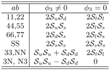
The flavor space trace in Eq. (37) can be easily per- formed. Since in the N−S basis the λa matrices have, with the exceptions of a = S, two nonzero matrix ele- ments, one generally obtains two terms which can cancel each other for some flavor combinations. The nonzero contributions are listed in Table II. In the case of the first three entries, the factor of 2 is the consequence of the identity

trD

ΓXSf(K)Γ⁰_YSf⁰(R)

=rXrY trD

ΓXSf⁰(−R)Γ⁰_YSf(−K)

, (38) which is applied inside the integral in Eq. (37) withY = X, followed by the shiftK→ −K. This identity can be proven using the cyclicity of the trace and that, given the charge conjugation operatorC=iγ²γ⁰,the matrices ΓX

of Table I satisfyCΓXC⁻¹ = rXΓ^T_X, where rX = 1 for X∈ {S, P, A}andrX=−1 forX =V.

We see from Table II that after the trace in flavor space is performed, depending on the indicesab, the self-energy (37) can be expressed either in terms of integrals involv- ing two different propagators

I^X(Q;m_f, m_f⁰) =−i 4

Z

K

tr_D

Γ_XSf(K)Γ⁰_XSf⁰(K−Q) , (39) or using integrals of the types already encountered in the one-flavor case (see Eq. (30)), obtained from Eq. (39) as

I^X(Q;m_f) = lim

m_f0→mf

I^X(Q;m_f, m_f⁰). (40)

TABLE II. Nonvanishing contributions to the self-energy (37) from the flavor space trace, tr

λaS¯0λbS¯0

, for φ3 6= 0 and their reduction in the isospin symmetric case, whereldenotes the light quarks with equal massesml≡mu=md.

ab φ36= 0 φ3= 0 11,22 2SuSd 2SlSl

44,55 2SuSs 2SlSs

66,77 2SdSs 2SlSs

SS 2SsSs 2SsSs

33,NN SuSu+SdSd 2SlSl

3N, N3 SuSu− SdSd 0

Being interested in the curvature mass, we evaluate the zero momentum self-energy, Π^(X)_ab ≡ Π^(X)_ab (Q = 0), expressing it in terms of the integrals

I^X(m1, m2)≡I^X(Q= 0;m1, m2),

I^X(m)≡I^X(Q= 0;m). (41) These are calculated in Appendix C, where, using partial fractioning and simple algebraic manipulations, they are reduced to a combination of simple integrals.

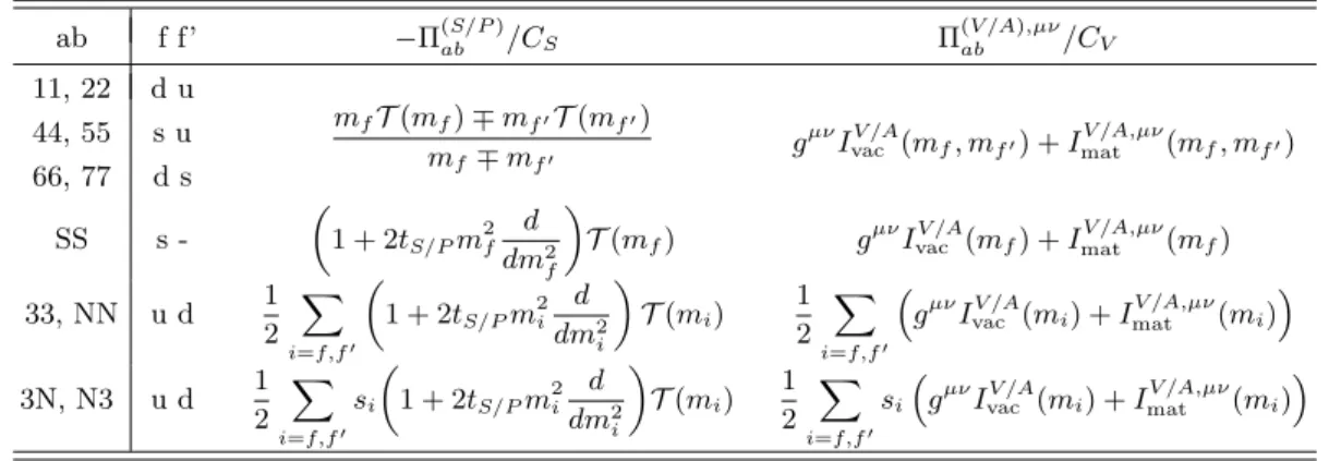
In the case of (pseudo)scalars the result is summarized in Table III, where we indicate the quark masses, labeled by f and f⁰, to be used in the formula of the one-loop self-energy for a given choice of the flavor indicesaandb.

The correction to the tree-level curvature mass ˆm^2,(S/P)_ab is of the form

Mˆ_ab^2,(S/P)= ˆm^2,(S/P)_ab + ∆ ˆm^2,(S/P)_ab +δmˆ^2,(S/P)_ab ,

∆ ˆm^2,(S/P_ab ⁾≡Π^(S/P)_ab,vac, δmˆ^2,(S/P_ab ⁾≡Π^(S/P_ab,mat⁾, (42) where the vacuum part needs renormalization and the matter part is finite and determined by T_f⁽¹⁾ (and its mass derivative, for some flavor indices). In some flavor cases Eq. (42) does not represent the physical curvature mass of the (pseudo)scalars, due to their mixing with (axial-)vectors. This issue is addressed in Sec. VI, where we will see that the mixing affects all the pseudoscalars, but only the scalars with flavor indices 4−7.

In the case of the (axial-)vectors, the evaluation of the self-energy requires some care. The self-energy is split intovacuum andmatter parts, as indicated in Table III.

For some flavor indices, namelya= 3,N,S forφ36= 0 and additionallya= 1,2 forφ₃ = 0, thevacuum part of the vector self-energy requires as in the N_f = 1 case, a co- variant calculation in a regularization scheme that com- plies with the requirement Π^(Vvac^),µν(Q = 0) = 0, which is familiar from QED. This requirement is investigated in Appendix B, where we relate it to a symmetry of the classical Lagrangian, which is manifest for a specific field background.

For simplicity, we use dimensional regularization to calculate the (axial-)vector self-energy, irrespective of the flavor index. The vacuum integral determining

the self-energy can be reduced to tadpole integrals (see Eq. (C12)). Its finite and divergent pieces are given in Eqs. (C9) and (C10). For thematter part we only need to consider purely temporal (00) and spatial (ij) com- ponents, as mixed (0i) components vanish due to sym- metric integration. The matter part of the relevant in- tegrals, given in Eqs. (C16) and (C17), contains also an integral whose mass derivative is proportional to the tad- pole, ^dU

(1) f

dm²_f =−³₂T_f⁽¹⁾ (see Eq. (A5)). In the equal mass limit this relation considerably simplifies the result.

A further complication with the (axial-)vectors is re- lated to the fact that one needs to consider the mode decomposition of the dressed propagator. This is done in Appendix E, using the usual set of tensors that in- cludes three- and four-dimensional projectors. As shown there, each mode has its own one-loop curvature mass, determined by the Lorentz components of the self-energy tensor in theQ→0 limit.

Using the form of the self-energy given in Table III in the expression (E11) that gives the contribution to a given mode p∈ {t,l,L}, one sees that the curvature mass has the structure

Mˆ_i,p^{2,(V /A)}= ˆm^{2,(V /A)}_i + ∆ ˆm^{2,(V /A)}_i +δpmˆ^{2,(V /A)}_i , (43) where i refers either to flavor indices (e.g. ab = 44) or to the particle (e.g. K1). ∆ ˆm²_i is the contribution of the vacuum part ∝ Ivac^{V /A}, which in view of Eq. (E11) is the same for all modes. δpmˆ²_i is the mode-dependent contribution of thematter part, and it is determined by

∝I_mat^{V /A,00} for the ‘l’ mode and ∝I_mat^{V /A,11} for the ‘t’ and

‘L’ modes, as discussed around Eqs. (E17) and (E19).

The ‘t’ and ‘l’ modes are, respectively, 3-transverse and 3-longitudinal, while the ‘L’ mode is 4-longitudinal. We will see in Sec. VI that the ‘L’ mode (43) influences the physical curvature mass of the (pseudo)scalars.

For the flavor indices appearing in the last three rows of Table III (and also forab = 11,22 for φ₃ = 0, when mu=md) one has only a matter fermionic contribution to the vector curvature mass and only in the case of the

’l’ mode. This is because the single mass integral is such thatI_vac^V (mf) =I_mat^V,11(mf) = 0,as shown in Appendix C.

In the isospin symmetric case the matter contributions to the curvature mass of the modes are (note that due to the absence of mixingω_N≡ω(782) andω_S≡φ(1020))

δtmˆ²_i =δLmˆ²_i = 0, i=ρ, ωN, ωS,

δlmˆ²_ρ/ωN =CVI_mat^V,00(ml), δlmˆ²_ωS =CVI_mat^V,00(ms), δt,Lmˆ²_K?=−Π^(V_44,mat^),11 =−CVI_mat^V,11(ml, ms),

δlmˆ²_K? = Π^(V_44,mat^),00 =CVI_mat^V,00(ml, ms) (44) for the vectors and

δ_t,Lmˆ²_a

1/f1N =−Π^(A),11_11,mat=−CVI_mat^A,11(m_l), δlmˆ²_a1/f1N = Π^(A),00_11,mat=CVI_mat^A,00(ml), δt,Lmˆ²_K1=−Π^(A),11_44,mat =−CVI_mat^A,11(ml, ms),

TABLE III. Fermionic contribution to the zero momentum one-loop self-energy of the scalar (S), pseudoscalar (P), vector (V) and axial-vector (A) fields in theφ36= 0 case. We indicate byf andf⁰the quark type whose mass has to be taken into account in the formula of the self-energy having flavor indicesab.Thematter part of the tadpole integralT(m) is given in Eq. (28) and the finite piece of thevacuum part in Eq. (56). Thevacuum integralIvac^{V /A} is given in Appendix C, together with the 00 and 11 components of thematter integralI_mat^{V /A,µν}. The constants areCS/V = 2Ncg²_S/V,tS= 1, tP = 0,andsu/d=±1.

ab f f’ −Π^(S/P_ab ⁾/CS Π^{(V /A),µν}_ab /CV

11, 22 d u

mfT(mf)∓mf⁰T(mf⁰)

mf∓m_f0 g^µνIvac^{V /A}(mf, mf⁰) +I_mat^{V /A,µν}(mf, mf⁰) 44, 55 s u

66, 77 d s SS s -

1 + 2tS/Pm²_f d dm²_f

T(mf) g^µνI_vac^{V /A}(mf) +I_mat^{V /A,µν}(mf) 33, NN u d 1

2 X

i=f,f⁰

1 + 2tS/Pm²_i d dm²_i

T(mi) 1 2

X

i=f,f⁰

g^µνI_vac^{V /A}(mi) +I_mat^{V /A,µν}(mi) 3N, N3 u d 1

2 X

i=f,f⁰

si

1 + 2t_S/Pm²_i d dm²_i

T(mi) 1 2

X

i=f,f⁰

si

g^µνI_vac^{V /A}(mi) +I_mat^{V /A,µν}(mi)

δlmˆ²_K1 = Π^(A),00_44,mat=CVI_mat^A,00(ml, ms), (45) for the axial-vectors, whereCV = 2Ncg_V² and for thef1S

meson the contributions are as forf1N withml replaced bym_s.The integrals are explicitly given in Appendix C.

The vacuum contributions need renormalization and their finite part is given forφ3= 0 in Eqs. (67) and (68).

B. Connection to previous calculations The fermionic correction to the (pseudo)scalar curva- ture masses was calculated first in Ref. [16] in the isospin symmetric case (φ3 = 0). The Polyakov-loop degrees of freedom were incorporated in Ref. [35]. Bringing the expression in Eq. (B12) of [16] and in Eq. (25) of [35]

in a form containing the tadpole and the bubble inte- gral at vanishing momentum is not mandatory, but it reveals the structure behind the obtained result for the curvature mass. Also, integration by parts shows that the result can be given in terms of a single function: the Fermi-Dirac distribution or the modified Fermi-Dirac dis- tribution (48), when Polyakov-loop degrees of freedom Φ and ¯Φ are included. This simple observation makes su- perfluous the introduction of B_f^± and C_f^±, used also in [7] following [35], and allows for a slight simplification of the formulas used so far in the literature.

Using the method of Ref. [16] we show below how to obtain the expressions of the (pseudo)scalar curvature masses given in Table III. The method assumes that in the ideal gas contribution of the three quarks to the grand potential we can use quark masses that depend on the fluctuating mesonic fields, as in Eq. (14) of the N_f = 1 case. The method works because forg_V = 0 and K = 0 the eigenvalues of the mass matrix in Eq. (D1) correspond to the u, d, and s quark sectors. In case of the (axial-)vectors, it is not enough to concentrate on the

mass matrix, as explained in Sec. I. Taking (axial-)vector field derivatives of the eigenvalues of the mass matrix, as in Ref. [17], results in a curvature mass tensor which breaks Lorentz covariance, as it is not proportional to gµν at T = 0.

Concentrating on the matter part of the grand poten- tial, we start from its expression given in the ideal gas approximation in Eq. (27) of [7]

Ω^(0)T_qq¯ (T, µ_q) =−2T X

f=u,d,s

Z d³p (2π)³

lng_f⁺(p)+lng⁻_f(p) , (46) where

g^±_f(p) = 1 + 3

Φ^±+ Φ^∓e^−βEf±(p)

e^−βEf±(p)+e^{−3βEf±(p)}, (47) with Φ⁺ = ¯Φ,Φ⁻ = Φ, E_f^±(p) = E_f(p)∓ µ_f and E²_f(p) = p²+M_f². Here M_f are the eigenvalues of the matrix in Eq. (D1), which depend not only on the scalar background, but also on the fluctuating (pseudo)scalar fields, generically denoted byϕa, withabeing the flavor index. After taking the second derivative with respect to ϕa, the fluctuating field is set to zero, in which case M_f(ϕ_a = 0) =m_f.

The modified Fermi-Dirac distribution functions F_f^±(p) = Φ^±e^−βEf±(p)+ 2Φ^∓e^{−2βE±f(p)}+e^{−3βEf±(p)}

g_f^±(p)

(48) are introduced by an integration by parts

T

Z d³p

(2π)³lng^±_f(p) = 1 2π²

Z ∞

0

dpp⁴F_f^±(p) E_f(p). (49) Then one uses that the dependence on ϕa is through

M_f²,which only appears in the combinationp²+M_f²,

∂

∂ϕ_a F_f^±(p) E_f(p) = 1

2p

∂

∂p

F_f^±(p) E_f(p)

∂M_f²

∂ϕ_a . (50) The above relation and integration by parts results in

∂²Ω^(0)T_qq¯ (T, µq)

∂ϕa∂ϕb

_ϕ=0

=−6X

f

∂²M_f²

∂ϕa∂ϕb

T_f⁽¹⁾

−∂M_f²

∂ϕa

∂M_f²

∂ϕb

B⁽¹⁾_f

ϕ=0

, (51) where the integralT_f⁽¹⁾≡ T⁽¹⁾(m_f) and its mass deriva- tive, defined in Eqs. (28) and (29), now contain the mod- ified Fermi-Dirac distribution functions (48).

Using Table III of [16] for the derivatives of the masses (Table II of [7] to also get the wave-function renormaliza- tion factors due to the shift of the (axial-)vector fields) one recovers the result obtained in [7] in the isospin sym- metric case, where one has mu,d = ml = gSφN/2. For example, in the ab = 11 scalar sector, which is not af- fected by the mixing, one has (Msdoes not contribute)

X

f=u,d

∂²M_f²

∂S1∂S1

_ϕ=0

=g_S², X

f=u,d

∂M_f²

∂S1

∂M_f²

∂S1

_ϕ=0

= 2g_S²m²_l, (52) so that the matter contribution of the fermions to the curvature mass obtained from Eq. (51) has the form

δm²_a0 =−6g_S²

T_l⁽¹⁾−2m²_lB_l⁽¹⁾

, (53) in accordance with Table III in view of (29).

The above simple calculation shows that in the pres- ence of Polyakov degrees of freedom the fermionic contri- bution to the curvature mass can be given in terms of the modified Fermi-Dirac distribution functions (48). Based on this, one can safely replace in our previous matter integralsf_f^±(p) withF_f^±(p).

V. RENORMALIZATION OF THE CURVATURE MASS

For simplicity, we discuss the renormalization of the fermionic correction to the curvature masses only in the isospin symmetric case (φ3 = 0) whereml ≡mu =md. Then, according to Table II, the contribution in the last row of Table III vanishes, while for 1−3, Nflavor indices one has to use the equal mass formula of thea= S case with the replacementms→ml.

Since the renormalization of the (pseudo)scalar cur- vature masses poses no problem and was already done in the literature, using dimensional regularization [36–

38] or cutoff regularization [7], we will only sketch an alternative method, which can be used in a localized ap- proximation, that is when the self-energy is evaluated at vanishing momentum.

The divergence(s) of a vacuum integral can be sepa- rated by expanding a localized propagator around the auxiliary function G0(K) = 1/(K²−M₀²), where M0

plays the role of a renormalization scale. For the tadpole integral, iterating once the identityG_f = G₀+ (m²_f − M₀²)G₀G_f,one obtains upon integration

T⁽⁰⁾(mf) =D2+m²_fD0+T_F⁽⁰⁾(mf), (54) where the first and second terms are the overall diver- gence and the subdivergence given in terms of

D₂=T⁽⁰⁾(M₀)−M₀²D₀, D₀= dT⁽⁰⁾(M₀)

dM₀² , (55) and the last term in Eq. (54) is finite,

T_F⁽⁰⁾(m_f) =i(m²_f−M₀²)² Z

K

G²₀(K)G_f(K)

= 1

16π²

M₀²−m²_f+m²_flnm²_f M₀²

. (56) With the above renormalization procedure the finite part of the tadpole is independent of whether covariant or noncovariant calculation, cutoff or dimensional regu- larization is used (provided the cutoff is sent to infinity in Eq. (56)). In a noncovariant calculation, Eq. (56) is obtained from Eq. (26) by writingEf(k) = (k²+M₀²+

∆m²_f)^1/2, with ∆m²_f =m²_f−M₀², and subtracting from thevacuum piece of the tadpole the first two terms ob- tained by expanding 1/Ef(k) in powers of ∆m²_f. Sub- tracting also the O (∆m²_f)²

term when renormalizing the integral

L⁽⁰⁾(m_f) =

Z d³k

(2π)³E_f(k), (57) which determines the one-loop fermionic contribution to the effective potential in Eq. (5) (and, with the replace- mentm²_f →Mˆ², also the contribution of the ring inte- grals with localized self-energy in Eq. (7)), results in the following finitevacuum part

L⁽⁰⁾_F (m_f) =− 1 64π²

∆m²_f 2m²_f+ ∆m²_f

−2m⁴_fln m²_f M₀²

, (58) which satisfies dL⁽⁰⁾_F (mf)/dm²_f =T_F⁽⁰⁾(mf),that is, the relation also holding between the unrenormalized inte- grals (57) and (26).

Now we turn our attention to the renormalization of the (axial-)vector curvature masses (43). The relevant terms of the ELσM Lagrangian introduced in Eq. (2) of Ref. [6] are those proportional to the coupling hi, i = 1,2,3 and the term containing the covariant derivative.

In dimensional regularization, used here withd= 4−2, no overall divergence is encountered, and thus the mass term of the (axial-)vectors∝m²₁is not needed. The tree- level mass squared of the vector and axial-vector fields de- pend on the strange and nonstrange scalar condensates