Popular Matchings in Complete Graphs
Ágnes Cseh1,2 · Telikepalli Kavitha3
Received: 9 April 2019 / Accepted: 1 December 2020
© The Author(s) 2021
Abstract
Our input is a complete graph G on n vertices where each vertex has a strict ranking of all other vertices in G. The goal is to construct a matching in G that is popular.
A matching M is popular if M does not lose a head-to-head election against any matching M′ : here each vertex casts a vote for the matching in {M,M�} in which it gets a better assignment. Popular matchings need not exist in the given instance G and the popular matching problem is to decide whether one exists or not. The popular matching problem in G is easy to solve for odd n. Surprisingly, the problem becomes 𝙽𝙿-complete for even n, as we show here. This is one of the few graph theoretic problems efficiently solvable when n has one parity and 𝙽𝙿-complete when n has the other parity.
Keywords Popular matching · Complexity · Stable matching
A preliminary version of this work appeared in FSTTCS 2018 [9].
Ágnes Cseh: Supported by the Federal Ministry of Education and Research of Germany (BMBF) in the KI-LAB-ITSE framework—project number 01IS19066, the Hungarian Academy of Sciences under its Momentum Programme (LP2016-3/2020), OTKA Grant K128611, and COST Action CA16228 European Network for Game Theory. Telikepalli Kavitha: This work was done while visiting the Hungarian Academy of Sciences, Budapest.
* Ágnes Cseh agnes.cseh@hpi.de
Telikepalli Kavitha kavitha@tifr.res.in
1 Centre for Economic and Regional Studies, Institute of Economics, Budapest, Hungary
2 Hasso Plattner Institute, University of Potsdam, Potsdam, Germany
3 Tata Institute of Fundamental Research, Mumbai, India
1 Introduction
Consider a complete graph G= (V,E) on n vertices where each vertex ranks all other vertices in a strict order of preference. Such a graph is called a roommates instance with complete preferences. The problem of computing a stable matching in G is classical and well-studied. Recall that a matching M is stable if there is no blocking pair with respect to M, i.e., a pair (u, v) where both u and v prefer each other to their respective assignments in M.
Stable matchings need not always exist in a roommates instance. For example, the instance given in Fig. 1 on 4 vertices d0,d1,d2,d3 has no stable matching. (Here d0 ’s top choice is d1 , second choice is d2 , and last choice is d3 , and similarly for the other vertices.)
Irving [20] gave an efficient algorithm to decide if G admits a stable matching or not. In this paper we consider a notion that is more relaxed than stability: this is the notion of popularity. For any vertex u, a ranking over neighbors can be extended naturally to a ranking over matchings as follows: u prefers matching M to matching M′ if (1) u is matched in M and unmatched in M′ or (2) u is matched in both and it prefers its partner in M to its partner in M′ . For any two matchings M and M′ , let 𝜙(M,M�) be the number of vertices that prefer M to M′.
Definition 1 Let M be any matching in G. M is popular if 𝜙(M,M�)≥𝜙(M�,M) for every matching M′ in G.
Suppose an election is held between M and M′ where each vertex casts a vote for the matching that it prefers. So 𝜙(M,M�) (similarly, 𝜙(M�,M) ) is the number of votes for M (resp., M′ ). A popular matching M never loses an election to another matching M′ since 𝜙(M,M�)≥𝜙(M�,M) : thus it is a weak Condorcet winner [5, 6]
in the corresponding voting instance. So popularity captures collective decision by the vertex set and it can be considered as a natural relaxation of stability.
The notion of popularity was first introduced in bipartite graphs in 1975 by Gärdenfors—popular matchings always exist in bipartite graphs since stable
Fig. 1 An instance that admits two popular matchings—marked by dotted blue and dashed orange edges—but no stable matching. The preference list of each vertex is illustrated by the numbers on its edges: a lower number indicates a more preferred neighbor (Color figure online)
matchings always exist here [13] and every stable matching is popular [14]. The proof that every stable matching is popular holds in non-bipartite graphs as well [4];
in fact, it is easy to show that every stable matching is a min-size popular match- ing [17]. Relaxing the constraint of stability to popularity allows us to find feasible matchings that may exist in instances that do not admit stable matchings; moreover, even when stable matchings exist, there may be popular matchings that achieve more
“social good” (such as larger size), which might be relevant in many applications.
Observe that the instance in Fig. 1 has two popular matchings:
M1= {(d0,d1),(d2,d3)} and M2= {(d0,d2),(d1,d3)} . However as was the case with stable matchings, popular matchings also need not always exist in the given instance G. Just take, for example, the same instance as in Fig. 1, but without vertex d0 . A complete graph G on an even number of vertices that has no popular matching is also easy to describe: take two copies of this instance on 3 vertices, i.e., d1,d2,d3 with preferences as given in Fig. 1 (without vertex d0 ) and three more vertices d′
1,d′
2,d′
3 whose preferences are analogous to d1,d2,d3 , respectively.
Since the instance has to be complete, add d1,d2,d3 (similarly, d′
1,d′
2,d′
3 ) at the tail of preference lists of d′
1,d′
2,d′
3 (resp., d1,d2,d3 ) in some arbitrary order. It is easy to check that this instance on 6 vertices has no popular matching.
The popular roommates problem is to decide if G admits a popular matching or not. When the graph is not complete, it is known that the popular roommates problem is 𝙽𝙿-complete [11, 15]. Here we are interested in the complexity of the popular roommates problem when the input instance is complete.
Interestingly, several popular matching problems that are intractable in bipar- tite graphs become tractable in complete bipartite graphs. The min-cost popu- lar matching problem in bipartite graphs is such a problem—this is 𝙽𝙿-hard in a bipartite graph with incomplete lists [11], however it can be solved in polynomial time in a bipartite graph with complete lists [8]. The difference is due to the fact that while there is no compact extended formulation of the convex hull of edge incidence vectors of all popular matchings in a general bipartite graph [10], this polytope has a compact extended formulation in a complete bipartite graph.
It is a simple observation (see Sect. 2) that when n is odd, a matching in a complete graph G on n vertices is popular only if it is stable. Since there is an efficient algorithm to decide if G admits a stable matching or not, the popular roommates problem in a complete graph G can be efficiently solved when n is odd. We show the following result here.
Theorem 1 Let G be a complete graph on n vertices, where n is even. The problem of deciding whether G admits a popular matching or not is 𝙽𝙿-complete.
So the popular roommates problem with complete preference lists is 𝙽𝙿-com- plete for even n while it is easy to solve for odd n. Some problems possess an inherently different nature depending on the parity of some characteristic input parameter, such as Latin squares [21] or various problems in voting [12]. Popular matchings do not belong to this set of problems—note that the popular room- mates problem is non-trivial for every n≥5 , i.e., there are both “yes instances”
and “no instances” of size n. It is rare and unusual for a natural decision problem in combinatorial optimization to be efficiently solvable when n has one parity and become 𝙽𝙿-complete when n has the other parity. We are not aware of any natural optimization problem on graphs that is non-trivially tractable when the cardinal- ity of the vertex set has one parity, which becomes intractable for the other parity.
1.1 Background and related work
The first polynomial time algorithm for the stable roommates problem was given by Irving [20] in 1985. Roommates instances that admit stable matchings were charac- terized in [30]. New polynomial time algorithms for the stable roommates problem were given in [29, 31].
Algorithmic questions for popular matchings in bipartite graphs have been well- studied in the last decade [1, 8, 17, 19, 22–24]. Not much was known on popular matchings in non-bipartite graphs. Biró et al. [1] proved that validating whether a given matching is popular can be done in polynomial time, even when ties are pre- sent in the preference lists. It was shown in [18] that every roommates instance on n vertices admits a matching with unpopularity factor O(logn) and that it is 𝙽𝙿-hard to compute a least unpopularity factor matching. It was shown in [19] that computing a max-weight popular matching in a roommates instance with edge weights is 𝙽𝙿 -hard, and more recently, that computing a max-size popular matching in a room- mates instance is 𝙽𝙿-hard [3].
The complexity of the popular roommates problem was open for several years [1, 7, 18, 19, 27] and two independent 𝙽𝙿-completeness proofs [11, 15] of this problem were shown very recently. Interestingly, both these hardness proofs need “incom- plete preference lists”, i.e., the underlying graph is not complete. The reduction in [15] is from a variant of the vertex cover problem called the partitioned vertex cover problem and we discuss the reduction in [11] in Sect. 1.2 below. So the complexity status of the popular roommates problem in a complete graph was an open problem and we resolve it here.
An interpretation of roommate instances with complete preference lists might be that each vertex finds every other vertex acceptable, or that being matched to any vertex is better than being unmatched, or that there is no outside option and the agents are all obliged to be matched within the market. Computational hardness for instances with complete lists has been investigated in various matching prob- lems under preferences. An example is the three-sided stable matching problem with cyclic preferences: this involves three groups of participants, say, men, women, and dogs, where dogs have strictly ordered preferences over men only, men have preferences over women only, and finally, women only list the dogs. If these prefer- ences are allowed to be incomplete, the problem of finding a weakly stable match- ing is known to be 𝙽𝙿-complete [2]. Until very recently, it had been one of the most intriguing open questions in stable matchings [27, 32] as to whether the same prob- lem becomes tractable when lists are complete. Lam and Plaxton gave a hardness proof for complete preference lists very recently, disproving the published conjec- tures [26].
1.2 Techniques
The 1-in-3 SAT problem is a well-known 𝙽𝙿-complete problem [28]: it consists of a Boolean formula B in CNF where every clause has 3 literals (none negated) and the problem is to find a satisfying truth assignment to the variables in B such that every clause has exactly one literal set to 𝗍𝗋𝗎𝖾 . We show a polynomial time reduc- tion from 1-in-3 SAT to the popular roommates problem with complete lists.
Our construction is based on the reduction in [11] that proved the 𝙽𝙿-complete- ness of the popular roommates problem. However there are several differences between our reduction and the reduction in [11]. The reduction in [11] considered a popular matching problem in bipartite graphs called the “exclusive popular set”
problem and showed it to be 𝙽𝙿-complete—when preference lists are complete, this problem can be easily solved. Thus the reduction in [11] needs incomplete preference lists.
The exclusive popular set problem asks if there is a popular matching in the given bipartite graph where the set of matched vertices is S, for a given even- sized subset S. A key step in the reduction in [11] from this problem in bipartite graphs to the popular matching problem in non-bipartite graphs merges all ver- tices outside S into a single node. Thus the total number of vertices in the non- bipartite graph used in [11] is odd. Moreover, the fact that popular matchings always exist in bipartite graphs is crucially used in this reduction. However in our setting, the whole problem is to decide if any popular matching exists in the given graph—thus there are no popular matchings that “always exist” here.
The reduction in [11] primarily uses the LP framework of popular matchings in bipartite graphs from [22, 23, 25] to analyze the structure of popular matchings in their instance. The LP framework characterizing popular matchings in non- bipartite graphs is more complex [25], so we use the combinatorial characteriza- tion of popular matchings [17] in terms of forbidden alternating paths/cycles to show that any popular matching in our instance will yield a 1-in-3 satisfying truth assignment for B. To show the converse, we use a dual certificate similar to the one used in [11] to prove the popularity of the matching that we construct using a 1-in-3 satisfying truth assignment for B.
Organization of the paper We discuss preliminaries in Section 2. Section 3 describes the construction of our complete graph G corresponding to a given 1-in-3 SAT formula B. Section 4 studies the structure of the graph G and Sec- tion 5 shows that any popular matching in G yields a 1-in-3 satisfying truth assignment for B. Section 6 completes the reduction by showing how to obtain a popular matching in G from any 1-in-3 satisfying truth assignment for B.
2 Preliminaries
This section contains a characterization of popular matchings from [17]. We also include a simple proof of the claim stated in Section 1 that when n is odd, every popular matching in G has to be stable.
Let M be any matching in G= (V,E) . For any pair (u,v) ∉M , define 𝗏𝗈𝗍𝖾
u(v,M) as follows: (here M(u) is u’s partner in M and M(u) =𝗇𝗎𝗅𝗅 if u is unmatched in M)
Label every edge (u, v) that does not belong to M by the pair (𝗏𝗈𝗍𝖾
u(v,M),𝗏𝗈𝗍𝖾
v(u,M)) . Thus every non-matching edge has a label in {(±,±)} . For example, if we consider the matching marked by the dashed orange edges in Fig. 1, then (d1,d2) is labeled (+,+) , (d2,d3) is labeled (+,−) , (d0,d1) is labeled (+,−) , and (d0,d3) is labeled (−,−) . Note that an edge is labeled (+,+) if and only if it is a blocking edge to M.
We remind the reader that an alternating path/cycle with respect to M is a path/cycle whose alternate edges belong to M: thus edges in this path/cycle alternate between belonging to the matching M and not belonging to the matching M. Let GM be the sub- graph of G obtained by deleting edges labeled (−,−) from G. The following theorem characterizes popular matchings in G.
Theorem 2 ([17]) M is popular in G if and only if GM does not contain any of the following with respect to M:
(1) an alternating cycle with a (+,+) edge;
(2) an alternating path with two distinct (+,+) edges;
(3) an alternating path with a (+,+) edge and an unmatched vertex as an endpoint of the path.
Using the above characterization, it can be easily checked whether a given matching is popular or not [17]. Thus our 𝙽𝙿-hardness result implies that the popular roommates problem with complete preferences is 𝙽𝙿-complete.
When n is odd. Recall the claim made in Sect. 1 that when n is odd, every popular matching in G has to be stable. A simple proof of this statement is included below.
Observation 1 ([16]) Let G be a complete graph on n vertices, where n is odd. Any popular matching in G has to be stable.
Proof Since n is odd and G is complete, any popular matching leaves exactly one vertex unmatched. Let M be a popular matching and let v be the vertex left unmatched in M. Consider a vertex u adjacent to v. We know that (u,w) ∈M for some w∈V⧵{v} , and due to Part (3) in Theorem 2, no (+,+) edge is incident to w.
Since v is adjacent not only to u, but to all vertices in the graph, this holds for all w∈V , i.e., there is no (+,+) edge incident to any vertex. Thus M is stable. ◻
𝗏𝗈𝗍𝖾u(v,M) =
{+ ifuprefersvtoM(u);
− ifuprefersM(u)tov.
3 The graph G
Recall that B is the input formula to 1-in-3 SAT. We assume that B has 𝜅 varia- bles X1,…,X𝜅 . The graph G that we construct here consists of gadgets in 4 levels along with 2 special gadgets that we will call the D-gadget and Z-gadget. Gadgets in level 1 correspond to variables in the formula B while gadgets in levels 0, 2, and 3 correspond to clauses in B. Variants of the gadgets in levels 0-3 and the D-gadget were used in [11] while the Z-gadget is new.
An overview We will first show that any popular matching M in G uses only intra- gadget edges. Every gadget will be in one of the following two states in M: stable state or unstable state. A gadget is in stable state if and only if there is no edge e with both its endpoints in this gadget such that e blocks M. Our aim is to show that for every clause c in B, the gadget of exactly one of the three variables in c is in unstable state in M—this will translate to a 1-in-3 satisfying truth assignment for B.
Preferences will be set such that unstable (similarly, stable) states of gadgets in one level force a certain number of gadgets in the adjacent level to be in unsta- ble (resp., stable) state. The reduction in [11] is also based on the same idea and for each clause in B, it used three level 0 gadgets, three level 2 gadgets, and one level 3 gadget (recall that clause gadgets are in levels 0, 2, 3). In our setting of complete preference lists, we will need “duplicates” or counterparts of all these gadgets to show the above reduction. So for each clause, we will use six level 0 gadgets, six level 2 gadgets, and two level 3 gadgets. In order to use Theorem 2, we will also need a new gadget to “glue” alternating paths across gadgets: this role will be performed by the Z-gadget which will be in stable state in M.
We will show that every level 3 gadget has to be in unstable state in M. Our technical lemma (Lemma 8) proves that this forces either two of the first three level 2 gadgets or two of the last three level 2 gadgets of every clause to be unsta- ble state in M. We then show this forces at least one gadget of the three variables in every clause in B to be in unstable state in M.
We also show that every level 0 gadget has to be in stable state in M. This will induce at most one gadget of the three variables in every clause in B to be in unstable state in M. Thus exactly one gadget of the three variables in every clause in B will be in unstable state in M.
Our gadgets We will now describe all the gadgets that we use here: along with a figure, we provide the preference lists of vertices in this gadget. The tail of each list consists of all vertices not listed yet, in an arbitrary order. Even though the preference lists are complete, the structure of the gadgets and the preference lists will ensure that inter-gadget edges will not belong to any popular matching, as we will show in Section 4.
The D-gadget The D-gadget is on 4 vertices d0,d1,d2,d3 and the preference lists of these vertices are as given in Fig. 1 with all vertices outside the D-gadget at the tail of each list (in an arbitrary order). Recall that this gadget admits no stable matching. The role of D-gadget will be that of a delimiter—we will show that every vertex will have to be matched in any popular matching to a neighbor preferred to all its neighbors in the D-gadget.
We describe gadgets from level 1 first, then levels 0, 2, 3, and finally, the Z-gadget. The stable matchings within the gadgets are highlighted by colors in the figures. The gray elements in the preference lists denote vertices that are outside this gadget. We will assume that D in a preference list stands for d0>d1>d2>d3.
Level 1 For each variable Xi in the formula B, we construct a gadget on four verti- ces as shown in Fig. 2.
The bottom vertices x′i and y′i will be preferred by some vertices in level 0 to vertices in their own gadget, while the top vertices xi and yi will be preferred by some vertices in level 2 to vertices in their own gadget. All four vertices in a level 1 gadget prefer to be matched among themselves, along the four edges drawn than be matched to any other vertex in the graph. This gadget has a unique stable matching {(xi,yi),(x�i,y�i)}
Level 0 For each clause . c=Xi∨Xj∨Xk in the formula B, we create 6 gadgets in level 0. For every ordered pair of elements in {i,j,k} , there is one such gadget. One of these gadgets (this corresponds to the pair (j, k)) can be seen in Fig. 3. The top two vertices, i.e. ac
1 and bc
1 , rank y′j and xk′ in level 1, as their respective second choices. Recall that indices j and k are well-defined in the clause c=Xi∨Xj∨Xk . Within this level 0 gadget on ac1,bc1,ac2,bc2 , both {(ac1,bc1),(ac2,bc2)} and {(ac1,bc2),(ac2,bc1)} are stable matchings. In the preference lists below (and also for
gadgets in levels 2 and 3), we have omitted the superscript c in their lists for the sake of readability.
The gadget on vertices {
ac3,ac4,bc3,bc4}
is built analogously: the vertex ac3 ranks y′k as its second choice, while bc3 ranks x′i second. In the third gadget, the vertex ac5 ranks y′i second, while bc5 ranks x′j second. Observe the shift in i, j, k indices as second choices for vertices ac
1,ac
3,ac
5 (and similarly, for bc
1,bc
3,bc
5).
The fourth, fifth, and sixth gadgets are analogous to their counterparts, the first, second, and third gadgets, respectively, but there is a slight twist. More pre- cisely, the preferences of a′c
1,a′c
2,b′c
1,b′c
2 in the fourth gadget are analogous to the preferences in Fig. 3, except that a′c
1 ranks y′k second, while b′c
1 ranks x′j second.
Fig. 2 The variable gadget in level 1
Fig. 3 A clause gadget in level 0. The set of preference lists on the left belongs to the first gadget, while the set of preference lists on the right belongs to the fourth gadget (this corresponds to the pair (k, j))
Similarly, the second choice of a′c
3 is y′i , the second choice of b′c
3 is x′k , and finally, a′c
5 ranks y′j second, while b′c
5 ranks x′i second. Observe the change in orientation of the indices i, j, k as second choice neighbors when comparing the first three level 0 gadgets of c with its last three level 0 gadgets. This will be important to us later.
Level 2 For each clause c=Xi∨Xj∨Xk in the formula B, we create 6 gadgets in level 2. The first gadget in level 2 is on vertices pc
0,pc
1,pc
2,qc
0,qc
1,qc
2 and their preference lists are described in Fig. 4. Note that pc
2 ranks yj from level 1 as its second choice, while qc
2 ranks xk from level 1 second.
The second gadget in level 2 is on vertices pc
3,pc
4,pc
5,qc
3,qc
4,qc
5 and it is built analo- gously. That is, pc
3 and qc
3 are each other’s top choices and similarly, pc
4 and qc
4 are each other’s top choices, and so on. The preference list of pc
5 is qc
3>yk>qc
4>qc
5>D>… and the preference list of qc
5 is pc
4>xi>pc
3>pc
5>D>… The third gadget in level 2 is on vertices pc
6,pc
7,pc
8,qc
6,qc
7,qc
8 and it is built anal- ogously. In particular, the preference list of pc
8 is qc
6>yi>qc
7>qc
8>D>… and the preference list of qc
8 is pc
7>xj>pc
6 >pc
8>D>… The fourth gadget in level 2 is on vertices p′c
0,p′c
1,p′c
2,q′c
0,q′c
1,q′c
2 and it is totally analogous to its counterpart, the first gadget in level 2. That is, p′c
0 and q′c
0 are each other’s top choices and similarly, p′c
1 and q′c
1 are each other’s top choices, and so on. In particular, the preference list of p′c
2 is q�c
0 >yj>q�c
1 >q�c
2 >D>… and the preference list of q′c
2 is p�c
1 >xk>p�c
0 >p�c
2 >D>… Similarly, the fifth gadget in level 2 is on vertices p′c
3,p′c
4,p′c
5,q′c
3,q′c
4,q′c
5 and it is totally analogous to the second gadget in level 2. Also, the sixth gadget in level 2 is on vertices p′c
6,p′c
7,p′c
8,q′c
6,q′c
7,q′c
8 and it is totally analogous to the third gadget in level 2.
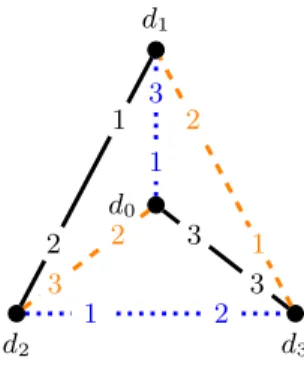
Level 3 For each clause c=Xi∨Xj∨Xk in the formula B, we create 2 gadgets in level 3. The first gadget is on vertices sc
0,sc
1,sc
2,sc
3,tc
0,tc
1,tc
2,tc
3 and the preference lists of these vertices are described in Fig. 5.
The counterpart of the first gadget in level 3 is the second gadget in level 3. It is on vertices s′c
0,s′c
1,s′c
2,s′c
3,t′c
0,t′c
1,t′c
2,t′c
3 and their preference lists are totally analo- gous to the preference lists of the first gadget in level 3.
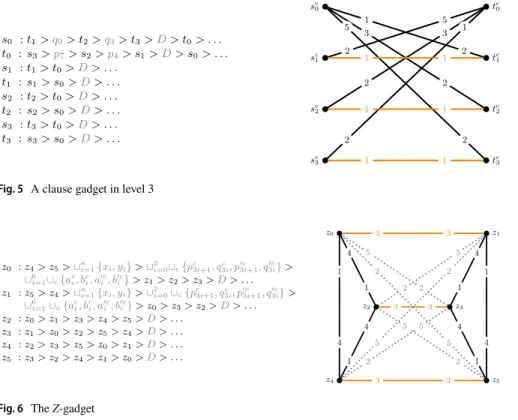
The Z-gadget. The Z-gadget is on 6 vertices z0,z1,z2,z3,z4,z5 and the prefer- ence lists of these vertices are given in Fig. 6. The vertices in a set stand for all
Fig. 4 A clause gadget in level 2
these vertices in a fixed arbitrary order. For example, ∪𝜅
i=1
{xi,yi}
denotes all the
“top” vertices belonging to all the 𝜅 variable gadgets in a fixed arbitrary order.
Note that G is a complete graph on an even number of vertices and so every pop- ular matching in G has to be a perfect matching.
4 Popular edges in G
Call an edge e in G popular if there is a popular matching M in G such that e∈M . In this section we identify edges that cannot be popular and show that every popular edge has to be an intra-gadget edge, i.e., it connects two vertices of the same gadget.
The following observation, which is straightforward, will be used repeatedly in our proofs.
Observation 2 Let v be u’s top choice neighbor. If v is matched in M to a neighbor worse than u then (u, v) is a blocking edge to M.
We now start restricting the set of edges that can possibly occur in a popular matching. Our first lemma eliminates some of the inter-gadget edges incident to ver- tices sc0 , tc0 , s′c0 , and t′c0 in level 3.
Fig. 5 A clause gadget in level 3
Fig. 6 The Z-gadget
Lemma 1 For any clause c, no popular matching in G can match sc
0 (similarly, tc
0) to a neighbor worse than tc
0 (resp., sc
0). An analogous statement holds for s′c
0 and t′c
0. Proof Let M be a popular matching such that (sc
0,v) ∈M for some vertex v such that tc
0>v in sc
0 ’s list, i.e., sc
0 prefers tc
0 to v. We claim this implies:
– a (+,+) edge reachable from v via an alternating path in GM that begins with a non-matching edge incident to v and
– a (+,+) edge reachable from sc
0 via an alternating path in GM that begins with a non-matching edge incident to sc
0.
If this is the same (+,+) edge then we have an alternating cycle in GM with a (+,+) edge, a contradiction to M’s popularity (by Theorem 2). If these are two different (+,+) edges then there is an alternating path in GM with two (+,+) edges, again a contradiction to M’s popularity (by Theorem 2).
(1) If v is a top choice neighbor for some vertex (such as xi,yi,zj for 1≤i≤𝜅 , 0≤j≤5 or d1,d2,d3 or ar𝓁,br𝓁,pr3h,pr3h+1,qr3h,qr3h+1 or their counterparts for 1≤𝓁≤6 , 0≤h≤2 and any clause r) then there is a (+,+) edge incident to v
(by Observation 2).
(2) Suppose v is one of sr0,tr0,s′r0,t0′r for some clause r (note that r≠c in the case of sr0,t0r ). Assume without loss of generality that v=sr0 . Then either (sr0,t0r) is a (+,+) edge or tr0 is matched in M to a neighbor better than sr0 . Recall tr0 ’s prefer- ence list: every vertex that t0r prefers to sr0 is either a top choice neighbor or it is d0 . In the former case, there is a (+,+) edge incident to t0r ’s partner (by Obser- vation 2) and in the latter case also there is a (+,+) edge incident to d0 since one of d1,d2,d3 is matched to a neighbor worse than d0 and so there is a (+,+) edge between this vertex in the set {d1,d2,d3} and d0 . Since the edge (sr0,t0r) is a (+,−) edge, there is a (+,+) edge reachable from v=sr0 via an alternating path of length 2.
(3) The only case left is when v is neither a top choice neighbor of some vertex nor one of sr0,tr0,s′r0,t0′r for some clause r. So v is a vertex such as d0 or x′i,y′i (for 1≤i≤𝜅 ) or pr3h+2,qr3h+2,p�r3h+2,q�r3h+2 (for h=0, 1, 2 and some clause r). It is easy to see that there is a (+,+) edge reachable from v via an alternating path of length at most 2. For instance, either (x�i,y�i) is a (+,+) edge or (xi,y�i) ∈M which creates the alternating path (sc0,x�i) − (y�i,xi) − (yi,∗) , where (xi,yi) is a (+,+) edge.
Similarly, we can argue that there is a (+,+) edge reachable from sc
0 via an alternat- ing path in GM . If tc
0 is matched to a neighbor worse than sc
0 then the edge (sc
0,tc
0) is a (+,+) edge. Else tc
0 is matched to a neighbor u better than sc
0 and this means there is a (+,+) edge incident to u, as we argued above in case (2). Hence there is a (+,+) edge reachable from sc
0 via an alternating path of length at most 2 in GM . ◻ Next we show that no inter-gadget edge incident to any vertex in the D-gadget can appear in any popular matching.
Lemma 2 Every popular matching matches the vertices in the D-gadget among themselves.
Proof Let M be a matching that matches di for some i∈ {0, 1, 2, 3} to a vertex v outside the D-gadget. This means at least 2 vertices di and dj in the D-gadget are matched to vertices outside the D-gadget. So (di,dj) is a (+,+) edge. We now claim there is a forbidden alternating path or cycle (as given in Theorem 2) to M’s popularity.
If v is a top choice neighbor or a vertex such as x′i,y′i (for 1≤i≤𝜅 ) or pc
3h+2,qc
3h+2,p�c
3h+2,q�c
3h+2 (for h=0, 1, 2 and some clause c) then there is a (+,+) edge e reachable from v via an alternating path of length at most 2 as seen in the proof of Lemma 1. This creates an alternating path in GM with 2 (+,+) edges: (dj,di) and e.
The other possibility is that v is sc
0,tc
0,s′c
0,t′c
0 for some clause c. Assume without loss of generality that v=sc
0 . Consider the vertex tc
0 . We know from Lemma 1 that tc
0 has to be matched to a neighbor at least as good as sc
0 . So we have the following cases:
(1) tc
0 is matched to dj in the D-gadget: this means there is either an alternating path with 2 (+,+) edges or an alternating cycle with a (+,+) edge:
If sc1 is matched to a neighbor worse than tc0 then the former is an alternating path with two (+,+) edges: these are (di,dj) and (tc0,sc1) . Else sc1 is matched to tc1 and the latter is an alternating cycle with a (+,+) edge, which is (di,dj).
(2) tc0 is matched to sci for some i∈ {1, 2, 3} : this means tci is matched to a neighbor worse than sc0 and so (sc0,tci) is a (+,+) edge and thus we have the following alter- nating path with two (+,+) edges (tic,sc0) and (di,dj) :
(3) tc0 is matched to either pc4 or pc7 : we will show that this results in an alternating path with two (+,+) edges. Assume without loss of generality that tc0 is matched to pc4 . Consider the following alternating path:
Recall that sc3 is the top choice neighbor of tc0 and the vertex pc4 is the top choice neighbor of qc5 . If the vertex sc3 is matched to a neighbor worse than tc0 then the former path is an alternating path in GM with two (+,+) edges in it: these are (sc3,tc0) and (pc4,qc5) . Else (sc3,tc3) ∈M and recall that the edge (sc0,tc3) is a (+,−)
(sc0,di)(+,+)− (dj,tc0)(+,+)− (sc1,∗) or
(sc0,di)(+,+)− (dj,tc0)(+,−)− (sc1,tc1)(−,+)− (sc0,di).
(∗,tic)(+,+)− (sc0,di)(+,+)− (dj,∗).
(∗,sc3)(+,+)− (tc0,pc4)(+,+)− (qc5,∗) or
(∗,dj)(+,+)− (di,sc0)(+,−)− (tc3,sc3)(−,+)− (tc0,pc4)(+,+)− (qc5,∗).
edge as sc
0 prefers tc
3 to di . This creates the latter path which is an alternating path in GM with 2 (+,+) edges in it: these are (di,dj) and (pc
4,qc
5) . ◻
The gadget D admits 2 popular matchings: {(d0,d1),(d2,d3)} and {(d0,d2),(d1,d3)} . So if M is a popular matching then either {(d0,d1),(d2,d3)}⊂M
or {(d0,d2),(d1,d3)}⊂M.The following lemma further restricts the set of popular edges and this will be used repeatedly in our proof.
Lemma 3 Let (u, v) be an edge in G where both u and v prefer d0 to each other. Then (u, v) cannot be a popular edge.
Proof Let M be a popular matching in G that contains such an edge (u, v). We know from Lemma 2 that either {(d0,d1),(d2,d3)}⊂M or {(d0,d2),(d1,d3)}⊂M . So there is always a blocking edge (di,dj) ∈ {(d1,d3),(d1,d2)} to M.
Observe that both u and v cannot belong to the D-gadget as there is no such pair within D. If exactly one of u, v belongs to the D-gadget then (u, v) is not a popular edge (by Lemma 2). So neither u nor v belongs to the D-gadget and this implies that u prefers d0,d1,d2,d3 to v and symmetrically, v prefers d0,d1,d2,d3 to u.
Consider the following alternating cycle C with respect to M:
where (di�,di) and (dj,dj�) are edges from the D-gadget in M and (di,dj) is a blocking edge. Thus C is an alternating cycle in GM with a (+,+) edge. This contradicts the
popularity of M (by Theorem 2). ◻
Corollary 1 The edges (sc
0,tc
0) and (s�c
0,t�c
0) are not popular edges for any clause c.
Corollary 1 follows from Lemma 3 by setting u and v to sc
0 and tc
0 (similarly, s′c and t′c 0
0 ), respectively. Let us call u a level i vertex if u belongs to a level i gadget.
Lemma 4 further restricts the set of popular edges; the proof of this lemma con- sists of three main claims.
Lemma 4 No edge between a level i vertex and a level i+1 vertex is popular, for 0≤i≤2.
The proof of Lemma 4 follows from Claims 1–3 proved below.
Claim 1 There is no popular edge between a level 0 vertex and a level 1 vertex.
Proof Let M be a popular matching in G with such an edge, say (ac
1,y�j) , where c=Xi∨Xj∨Xk . We claim this would create an alternating path in GM with two (+,+) edges in it (this would contradict Theorem 2). Consider the vertex bc1 . There are 3 possibilities for bc1 ’s partner in M.
(u,v)(+,−)− (di�,di)(+,+)− (dj,dj�)(−,+)− (u,v),
(1) bc
1 is matched to ac So (ac 2
2,bc
2) is labeled (+,+) . Recall that bc
2 is ac
2 ’s top choice and the only neighbor that bc
2 prefers to ac
2 is ac
1 (which is matched to y′j ). Consider the follow- ing alternating path in GM∶
If x′j is matched to a neighbor worse than y′j then the above is an alternating path in GM with two (+,+) edges: these are (bc
2,ac
2) and (y�j,x�j) . Else replace (x�j,∗) in the above path with (x�j,yj) − (xj,∗) : the (+,+) edges here are (bc2,ac2) and (yj,xj). (2) bc
1 is matched to x′k
Either the edge (x�k,y�k) or the edge (xk,yk) will block M. Suppose y′k is matched to a neighbor worse than x′k in M. Consider the following alternating path in GM :
Either the above is an alternating path in GM with two (+,+) edges or by replacing (x�j,∗) with (x�j,yj) − (xj,∗) (as done in case (1)), we get an alternating path in GM with two (+,+) edges. If y′k is matched to a neighbor better than x′k in M, i.e., if (xk,y�k) ∈M then prefix both these alternating paths with (∗,yk) . This will yield an alternating path in GM with (xk,yk) as a blocking edge and either (x�j,y�j) or (xj,yj) as a blocking edge.
(3) bc
1 is matched to a neighbor worse than ac Then the edge (ac 1
1,bc
1) is labeled (+,+) . Consider the following alternating path in GM :
That is, if x′j is matched to a neighbor worse than y′j then consider the first alter- nating path above: this is an alternating path in GM with both (bc
1,ac
1) and (y�j,x�j) as (+,+) edges. Else (x�j,yj) ∈M and the second alternating path is an alternat- ing path in GM with (bc
1,ac
1) and (yj,xj) as (+,+) edges.
Thus (ac
1,y�j) cannot belong to any popular matching in G. Similarly, (bc
1,x�k) also cannot belong to any popular matching. Suppose (bc
1,x�k) ∈M . Consider the ver- tex ac
2 : there are 2 possibilities for ac
2 ’s partner in M.
(1) ac2 is matched to bc2
Recall that ac1 is bc2 ’s top choice and since ac1 is not matched to either y′j (by our proof above) or bc
1 (which is matched to x′k ), the edge (ac
1,bc
2) is labeled (+,+) . Consider the following alternating path in GM :
(∗,bc2)(+,+)− (ac2,bc1)(−,+)− (ac1,y�j)(+,+)− (x�j,∗).
(∗,y�k)(+,+)− (x�k,bc
1)(−,+)− (ac
1,y�j)(+,+)− (x�j,∗).
(∗,bc1)(+,+)− (ac1,y�j)(+,+)− (x�j,∗) or (∗,bc1)(+,+)− (ac1,y�j)(+,−)− (x�j,yj)(+,+)− (xj,∗).