CERS-IE WORKING PAPERS | KRTK-KTI MŰHELYTANULMÁNYOK
INSTITUTE OF ECONOMICS, CENTRE FOR ECONOMIC AND REGIONAL STUDIES, BUDAPEST, 2020
Understanding popular matchings via stable matchings
ÁGNES CSEH – YURI FAENZA – TELIKEPALLI KAVITHA – VLADLENA POWERS
CERS-IE WP – 2020/3
January 2020
https://www.mtakti.hu/wp-content/uploads/2020/01/CERSIEWP202003.pdf
CERS-IE Working Papers are circulated to promote discussion and provoque comments, they have not been peer-reviewed.
Any references to discussion papers should clearly state that the paper is preliminary.
Materials published in this series may be subject to further publication.
ABSTRACT
An instance of the marriage problem is given by a graph G together with, for each vertex of G, a strict preference order over its neighbors. A matching M of G is popular in the marriage instance if M does not lose a head-to-head election against any matching where vertices are voters. Every stable matching is a min-size popular matching; another subclass of popular matchings that always exist and can be easily computed is the set of dominant matchings. A popular matching M is dominant if M wins the head-to-head election against any larger matching. Thus every dominant matching is a max-size popular matching and it is known that the set of dominant matchings is the linear image of the set of stable matchings in an auxiliary graph.
Results from the literature seem to suggest that stable and dominant matchings behave, from a complexity theory point of view, in a very similar manner within the class of popular matchings.
The goal of this paper is to show that indeed there are differences in the tractability of stable and dominant matchings, and to investigate further their importance for popular matchings. First, we show that it is easy to check if all popular matchings are also stable, however it is co-NP-hard to check if all popular matchings are also dominant. Second, we show how some new and recent hardness results on popular matching problems can be deduced from the NP-hardness of certain problems on stable matchings, also studied in this paper, thus showing that stable matchings can be employed not only to show positive results on popular matching (as is known), but also most negative ones. Problems for which we show new hardness results include finding a min-size (resp. max-size) popular matching that is not stable (resp.
dominant). A known result for which we give a new and simple proof is the NP- hardness of finding a popular matching when G is non-bipartite.
JEL codes: C63, C78
Keywords: popular matching, NP-completeness, polynomial algorithm, stable
matching
Ágnes Cseh
Centre for Economic and Regional Studies, Institute of Economics, Tóth Kálmán utca 4., Budapest, 1097, Hungary
e-mail: cseh.agnes@krtk.mta.hu Yuri Faenza
IEOR, Columbia University, New York, USA;
e-mail: yf2414@columbia.edu Telikepalli Kavitha
Tata Institute of Fundamental Research, Mumbai, India e-mail: kavitha@tifr.res.in
Vladlena Powers
IEOR, Columbia University, New York, USA;
e-mail: yf2414@columbia.edu
Népszerű párosítások megértése stabil párosítások segítségével
ÁGNES CSEH – YURI FAENZA – TELIKEPALLI KAVITHA – VLADLENA POWERS
ÖSSZEFOGLALÓ
Adott egy páros gráf G = (A u B, E), ahol minden csúcs szigorú listában rangsorolja a szomszédjait. Egy M párosítást akkor nevezünk népszerűnek, ha nincsen olyan M’ párosítás, hogy több csúcs részesíti előnyben M’-t M-mel szemben, mint fordítva. Minden stabil párosítás minimális méretű népszerű párosítás, és egy másik, könnyen kiszámolható alosztálya a népszerű párosításoknak az úgynevezett domináns párosítások halmaza. Egy népszerű párosítást akkor nevezünk dominánsnak, ha az megnyer minden szavazást egy nálánál nagyobb méretű párosítással szemben. Ebből következik, hogy minden domináns párosítás egyben legnagyobb méretű népszerű párosítás is. Az is ismert, hogy a domináns párosítások megkaphatók egy kibővített input stabil párosításainak a lineáris leképezéseiként.
Cikkünkben megmutatjuk, hogy a stabil és a domináns párosításokkal kapcsolatos bonyolultsági eredmények igen különbözőek a két osztályra. Elsőként bebizonyítjuk, hogy könnyű ellenőrizni, hogy minden népszerű párosítás stabil-e, viszont coNP-nehéz eldönteni, hogy minden népszerű párosítás domináns-e. Ezután bemutatunk néhány NP-teljességi bizonyítást népszerű párosításokra, amik stabil párosításokra bizonyított eredményekből következnek. Ezzel demonstráljuk, hogy a stabilitásra bizonyított eredmények nemcsak a pozitív, de a nehézségi bizonyításokban is hasznosnak bizonyulnak. Az újonnan nehéznek besorolt problémák közt megtalálható a legkisebb nem stabil és a legnagyobb nem domináns párosítás találása. Népszerű párosítás létezésére nem páros gráfon adunk egy új és egyszerű bizonyítást.
JEL: C63, C78
Kulcsszavak: népszerű párosítás, NP-teljesség, polinomiális algoritmus, stabil párosítás
Understanding popular matchings via stable matchings
Agnes Cseh´ 1, Yuri Faenza2, Telikepalli Kavitha3?, and Vladlena Powers2
1 Centre for Economic and Regional Studies, Institute of Economics, Budapest, Hungary;
cseh.agnes@krtk.mta.hu
2 IEOR, Columbia University, New York, USA;{yf2414, vp2342}@columbia.edu
3 Tata Institute of Fundamental Research, Mumbai, India;kavitha@tifr.res.in
Abstract. An instance of the marriage problem is given by a graphG= (A∪B, E), together with, for each vertex ofG, a strict preference order over its neighbors. A matching M of G is popular in the marriage instance if M does not lose a head-to-head election against any matching where vertices are voters. Every stable matching is a min-size popular matching;
another subclass of popular matchings that always exist and can be easily computed is the set ofdominantmatchings. A popular matchingM is dominant ifM wins the head-to-head election against any larger matching. Thus every dominant matching is a max-sizepopular matching and it is known that the set of dominant matchings is the linear image of the set of stable matchings in an auxiliary graph. Results from the literature seem to suggest that stable and dominant matchings behave, from a complexity theory point of view, in a very similar manner within the class of popular matchings.
The goal of this paper is to show that indeed there are differences in the tractability of stable and dominant matchings, and to investigate further their importance for popular matchings.
First, we show that it is easy to check if all popular matchings are also stable, however it is co-NP hard to check if all popular matchings are also dominant. Second, we show how some new and recent hardness results onpopular matching problems can be deduced from the NP- hardness of certain problems onstablematchings, also studied in this paper, thus showing that stable matchings can be employed not only to show positive results on popular matching (as is known), but also most negative ones. Problems for which we show new hardness results include finding a min-size (resp. max-size) popular matching that is not stable (resp. dominant). A known result for which we give a new and simple proof is the NP-hardness of finding a popular matching whenGis non-bipartite.
1 Introduction
Consider a bipartite graphG= (A∪B, E) onnvertices andmedges where each vertex has a strict ranking of its neighbors. Such a graph supplied with preference lists, also called amarriageinstance, is an extensively studied model in two-sided matching markets. The problem of computing astable matching in Gis classical. A matchingM is stable if there is noblocking edge with respect toM, i.e., an edge whose endpoints prefer each other to their respective assignments inM. The notion of stability was introduced by Gale and Shapley [11] in 1962 who showed that stable matchings always exist inGand there is a simple linear time algorithm to find one.
Stable matchings in an instance with an underlying bipartite graph Gare well-understood [14], with efficient algorithms [19, 27, 9, 24, 10, 26] to solve several optimization problems that have many applications in economics, computer science, and mathematics. Here we study a related and more relaxed notion calledpopularity. This notion was introduced by G¨ardenfors [12] in 1975 who showed that every stable matching is also popular. For any vertexu, its preference over neighbors extends naturally to a preference over matchings as follows:uprefersM to M0 either if (i)uis matched in M and unmatched in M0 or (ii)u is matched in both and prefers its partner inM to its partner inM0. Letψ(M, M0) be the number of vertices that preferM toM0.
Definition 1. A matching M is popular if ψ(M, M0) ≥ψ(M0, M) for every matching M0 in G, i.e., ∆(M, M0)≥0 where∆(M, M0) =ψ(M, M0)−ψ(M0, M).
?Work done while visiting Max-Planck-Institut f¨ur Informatik, Saarbr¨ucken, Germany.
Hence, in a voting-based context, vertices constitute the set of voters, and each matching in the instance is an alternative. In a head-to-head election between two matchings, each vertex casts a vote for the matching that it prefers and it abstains from voting if its assignment is the same in both matchings. A popular matching, by definition, never loses such a head-to-head election against another matching. Hence, a popular matching is a weakCondorcet winner[3, 4] in the corresponding voting instance. It is easy to show that a stable matching is a min-size popular matching [16]. Thus larger matchings and more generally, matchings that achieve more social good, are possible by relaxing the constraint of stability to popularity.
Algorithmic questions for popular matchings in bipartite graphs have been well-studied in the last decade [2, 16, 20, 21, 17, 6, 8]. We currently know efficient algorithms for the following problems in bipartite graphs: (i) min-size popular matchings, (ii) max-size popular matchings, and (iii) finding a popular matching with a given edge. All these algorithms compute either a stable matching or a dominantmatching.
Definition 2. A popular matching M is dominant in G if M is more popular than any larger matching inG, i.e.,∆(M, M0)>0 for any matchingM0 such that|M0|>|M|.
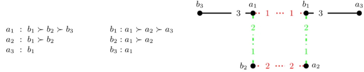
Thus a dominant matching defeats every larger matching in a head-to-head election, so it imme- diately follows that a dominant matching is a popular matching of maximum size. The example in Fig. 1 (from [16]) demonstrates the differences between stable, dominant, and max-size matchings.
In the graph G = (A∪B, E) here, we have A = {a1, a2, a3} and B = {b1, b2, b3}. The same preferences are depicted as numbers on the edges and as lists to the left of the drawn graph. Vertex b1 is the top choice for allai’s,b2is the second choice fora1anda2, andb3is the third choice fora1 alone. The preference lists of thebi vertices are symmetric. There are two popular matchings here, both of them have the same cardinality:M1={(a1, b1),(a2, b2)} andM2={(a1, b2),(a2, b1)}.
The matching M1 is stable, but not dominant, since it is not more popular than the larger matching M3 = {(a1, b3),(a2, b2),(a3, b1)}. Observe that in an election between M1 and M3, the vertices a1, b1 vote for M1, the vertices a3, b3 vote for M3, and the vertices a2, b2 are indifferent betweenM1andM3; thus∆(M1, M3) = 2−2 = 0. The matchingM2is dominant sinceM2 is more popular than M3: observe that ∆(M2, M3) = 4−2 = 2 sincea1, b1, a2, b2 prefer M2 to M3 while a3, b3preferM3to M2. HoweverM2is not stable, since (a1, b1) blocks it.
a1 : b1b2b3 b1:a1a2a3
a2 : b1b2 b2:a1a2
a3 : b1 b3:a1
a1
b2
b1
a2
b3 a3
2 1
1 1
3
2 2
1 2
3
Fig. 1.The above instance admits two popular matchings. The stable matching M1 is marked by dotted red edges, while the dominant matchingM2 is marked by dashed green edges.
Dominant matchings always exist in a bipartite graph [16] and a dominant matching can be computed in linear time [20]. Moreover, dominant matchings are the linear image of stable matchings in an auxiliary instance [6], hence oftentimes an optimization problem over the set of dominant matchings (e.g. finding one of maximum weight) boils down to solving the same problem on the set of stable matchings. Very recently, the following rather surprising result was shown [8]: it is NP-hard to decide if a bipartite graph admits a popular matching that isneither stable nor dominant.
1.1 Our problems, results, and techniques
Everything known so far about stable and dominant matchings seemed to suggest that those classes play somehow symmetric roles in popular matching problems in bipartite graphs: both classes are
always non-empty and one is a tractable subclass ofmin-size popular matchingswhile the other is a tractable subclass of max-size popular matchings. Our first set of results shows that this symmetry is not always the case.
Our starting point is an investigation of the complexity of the following two natural and easy- to-ask questions on popular matchings in a bipartite graphGwith strict preference lists:
(1) iseverypopular matching inGalso stable?
(2) iseverypopular matching inGalso dominant?
Both these questions are trivial to answer in instances that admit popular matchings of more than one size. Then the answer to both questions is “no” since {dominant matchings} ∩ {stable matchings}=∅ in such graphs as dominant matchings are max-size popular matchings while stable matchings are min-size popular matchings. Thus, in this case, a dominant matching is anunstable popular matching and a stable matching is anon-dominantpopular matching inG. However, when all popular matchings inGhave the same size, these questions are non-trivial.
Moreover, it is useful to ask these questions because when there are edge utilities, the problem of finding a max-utility popular matching is NP-hard in general [22] and also hard to approximate to a factor better than 2 [8]; however if every popular matching is stable (similarly, dominant), then the max-utility popular matching problem can be solved in polynomial time. Thus a “yes” answer to either of these questions has applications. We show the following dichotomy here: though both these questions seem analogous,only one is easy-to-answer.
(∗) There is anO(m2)algorithm to decide if every popular matching in G= (A∪B, E) is stable, however it is co-NP complete to decide if every popular matching inG= (A∪B, E)is dominant.
The first step in proving (∗) is to show that questions (1) and (2) are equivalent to the following:4 (10) is everydominant matching inGalso stable?
(20) is everystable matching inGalso dominant?
In Section 3, we give a combinatorial algorithm that solves (10) in time O(m2). We settle the complexity of (2) and (20) in Section 4, showing that the problem is co-NP hard. We deduce the latter from the hardness of finding a stable matching with a certain augmenting path: a result that is shown in this paper.
Our hardness reduction is surprisingly simple when compared to those that appeared in recent publications on popular matchings [8, 13, 22], and establishes a new connection between hardness of problems for stable matchings and hardness of problems for popular matchings. This connection turns out to be very fertile: we exploit it further to show NP-hardness of the following new deci- sion problems for a bipartite graph G(in particular, these hardness results are not implied by the reductions from [8, 13, 22]):
(3) is there a stable matching inGthat is dominant?
(4) is there a max-size popular matching inGthat is not dominant?
(5) is there a min-size popular matching inGthat is not stable?
A general graph (not necessarily bipartite) with strict preference lists is called a roommates instance. Popular matchings need not always exist in a roommates instance and the popular room- mates problem is to decide if a given instance admits one or not. The complexity of the popular roommates problem was open for close to a decade and very recently, two independent proofs of NP-hardness [8, 13] of this problem were shown. Both these proofs are rather lengthy and technical.
We use the hardness result for problem (3) to show a short and simple proof of NP-hardness of the popular roommates problem. Moreover, the hardness result for (5) shows an alternative and much simpler proof of NP-hardness (compared to [8]) of the following decision problem in a marriage
4 Although similar in spirit, the arguments leading from (1) to (10) and from (2) to (20) are not the same, see Lemma 2 and Lemma 3.
instanceG= (A∪B, E) equipped with strict preference lists: is there a popular matching inGthat is neither stable nor dominant?5
Algorithms for computing min-size/max-size popular matchings and for the popular edge prob- lem compute either stable matchings or dominant matchings. Dominant matchings inGare stable matchings in a related graph G0 (see Section 2) and so the machinery of stable matchings is used to solve dominant matching problems. Thus all positive results in the domain of popular matchings can be attributed to stable matchings. Conversely, all hardness results proved in this paper rely on the fact that it is hard to find stable matchings that have / do not have certain augmenting paths.
Hence, properties of stable matchings are also responsible for, and provide a unified approach to, the hardness of many popular matching problems.
1.2 Background and related results
In all problems considered in this paper, all vertices of a graph have strict preference lists over their neighbors. The first algorithmic question studied in the domain of popular matchings was in the one-sided preference lists model in bipartite graphs: here, unlike in our setting, one side of the graph consists of agents who have preferences over their neighbors while vertices on the other side are objects with no preferences. Popular matchings need not always exist here and an efficient algorithm was shown in [1] to determine if one exists or not.
Popular matchings always exist in bipartite graphs when every vertex has a strict preference list [12]. However when preference lists are not strict, the problem of deciding if a popular match- ing exists or not is NP-hard [2, 5]. The first non-trivial algorithms designed for computing popular matchings in bipartite graphs with strict preference lists were the max-size popular matching al- gorithms [16, 20]. These algorithms compute dominant matchings and the termdominant matching was formally defined a few years later in [6] to solve the “popular edge” problem.
As mentioned earlier, it was recently shown that it is NP-hard to decide if a marriage instance admits a popular matching that is neither stable nor dominant [8]. This hardness result was shown by a reduction from 1-in-3 SAT and a consequence of this hardness result was the hardness of the popular roommates problem. The NP-hardness of popular roommates problem shown in [13] was by a reduction from a problem called thepartitioned vertex coverproblem.
There are several efficient algorithms to solve the stable roommates problem [18, 25, 26]. In con- trast, thedominant roommatesproblem, i.e., the problem of deciding whether a roommates instance admits a dominant matching or not, is NP-hard [8]. Our NP-hardness proof of the popular room- mates problem also proves the hardness of the dominant roommates problem and it is much simpler than the proof in [8].
Organization of the paper. Section 2 contains known facts on popular, stable, and dominant match- ings, that will be used throughout the paper. In Section 3, we present an algorithm to decide if G has an unstable popular matching. Section 4 has our co-NP hardness result, which is deduced from the problem of deciding whether stable matchingswithcertain augmenting paths exist, whose hardness is also proved in Section 4. In Section 5 we show how the problem of deciding whether a stable matching without certain augmenting paths exists implies new and known hardness results, in particular the hardness of deciding if there exists a matching that is both stable and dominant.
2 Preliminaries
LetG= (A∪B, E) be the graph in our input. We will often refer to vertices in Aand B as men andwomen, respectively. We will always assume that each vertex has a strict preference order over his/her neighbors, and the set of these lists is denoted by P. An instance of our problem consists of Gand P, but we will omit to explicitly mention P when it is clear from the context. We often
5 The reduction in [8] also showed that it was NP-hard to decide ifGadmits a popular matching that is neither a min-size nor a max-size popular matching. Our reduction does not imply this.
abbreviaten =|A∪B| and m= |E|. We now sketch four important tools developed for popular matchings in earlier papers. Each of these will be used in later parts of this paper.
1) Characterization of popular matchings.LetM be any matching inG. For any edge (a, b)∈/ M, definevotea(b, M) as follows (hereM(a) isa’s partner in the matchingM andM(a) =nullifa is unmatched inM):
votea(b, M) =
(+ ifaprefersbtoM(a);
− ifaprefersM(a) tob.
We can similarly definevoteb(a, M). Label every edge (a, b)∈/ M by (votea(b, M),voteb(a, M)).
Thus every edge outsideM has a label in{(±,±)}. Note that an edgeeis labeled (+,+) if and only ifeis a blocking edge toM.
LetGM be the subgraph ofGobtained by deleting edges labeled (−,−) from G. The following theorem characterizes popular matchings. This characterization holds in non-bipartite graphs as well.
Theorem 1 ([16]). Matching M is popular in instance G,P if and only ifGM does not contain any of the following with respect toM:
(i) an alternating cycle with a(+,+) edge;
(ii) an alternating path with two distinct(+,+) edges;
(iii) an alternating path with a (+,+)edge and an unmatched vertex as an endpoint.
The following theorem characterizes dominant matchings.
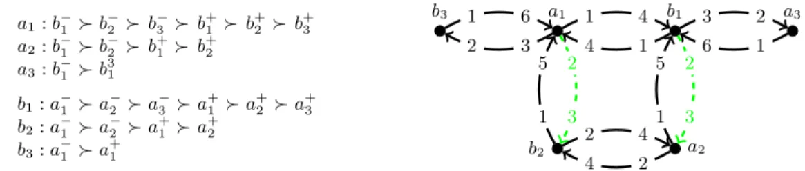
Theorem 2 ([6]). A popular matchingM is dominant iff there is noM-augmenting path inGM. 2) The graphG0.Dominant matchings inGare equivalent to stable matchings in a related graph G0: this equivalence was first used in [6], later simplified in [8]. The graphG0is the bidirected graph corresponding toG. The vertex set ofG0 is the same as the vertex setA∪B ofG and every edge (a, b) inGis replaced by 2 edges inG0: one directed from atobdenoted by (a+, b−) and the other directed frombtoadenoted by (a−, b+). Letu∈A∪Band supposev1v2· · · vk isu’s preference order inG. Thenu’s preference order inG0 is:
v1−v−2 · · · v−k v1+v2+· · · v+k.
That is, every vertex prefers outgoing edges to incoming edges and among outgoing edges, it maintains its original preference order and among incoming edges, it maintains again its original preference order. Observe that vertex preferences inG0 are expressed on incident edges rather than on neighbors. However it is easy to see that stable matchings inG0are equivalent to stable matchings in the following conventional graph that has 3 vertices u+, u−, d(u) corresponding to each vertex u in G0. The preference order of u+ is v−1 v−2 · · · vk− d(u), the preference order of u− is d(u)v1+v+2 · · · vk+, and the preference order ofd(u) isu+u−.
It was shown in [6, 8] that any stable matching M0 in G0 projects to a dominant matching M in G by setting (a, b) ∈M if and only if either (a+, b−) or (a−, b+) is in M0, and conversely, any dominant matching inGcan be realized as a stable matching inG0.
3) The set of matched vertices.We will be using theRural Hospitals Theoremfor stable match- ings (see e.g. [14]) that states that all stable matchings inGmatch the same subset of vertices. Note that every dominant matching in G matches the same subset of vertices (via the Rural Hospitals Theorem for stable matchings inG0). More generally, the following fact is true, whereV(N) is the set of vertices matched in a matchingN.
Lemma 1 ([15, 16]). Let S be a stable, M be a popular, and D be a dominant matching in a marriage instanceG= (A∪B, E),P. ThenV(S)⊆V(M)⊆V(D).
Thus, in particular, in instances where stable matchings have the same size as dominant match- ings, all popular matchings match the same subset of vertices.
4) Witness of a popular matching.Let ˜Gbe the graph Gaugmented with self-loops. That is, we assume each vertex is its own last choice neighbor. So we can henceforth regard any matching M in Gas a perfect matching ˜M in ˜Gby including self-loops at all vertices left unmatched in M. The following edge weight functionwtM in ˜Gwill be useful to us. For any edge (a, b) inG, define:
wtM(a, b) =
2 if (a, b) is labeled (+,+)
−2 if (a, b) is labeled (−,−) 0 otherwise.
We need to define wtM for self-loops as well: let wtM(u, u) = 0 ifu is matched to itself in ˜M, elsewtM(u, u) =−1. For any matchingN inG, it is easy to see thatwtM( ˜N) =∆(N, M) and soM is popular inGif and only if every perfect matching in ˜Ghas weight at most 0. Theorem 3 follows from LP-duality and the fact thatGis a bipartite graph.
Theorem 3 ([23, 21]). A matchingM in G= (A∪B, E),P is popular if and only if there exists a vectorα∈ {0,±1}n such that P
u∈A∪Bαu= 0,
αa+αb ≥ wtM(a, b) ∀(a, b)∈E and αu ≥ wtM(u, u) ∀u∈A∪B.
For any popular matching M, a vector α as given in Theorem 3 will be calledM’s witness or dual certificate. A popular matching may have several witnesses. Any stable matching has 0as a witness.
Call an edgeepopularif there is a popular matching inGthat containse. For any popular edge (a, b), it was shown in [7] (using complementary slackness) thatαa+αb=wtM(a, b). This will be a useful fact for us. Another useful fact from [7] (again by complementary slackness) is that if vertex uis left unmatched in some popular matching thenαu=wtM(u, u) for every popular matchingM; thusαu= 0 ifuis left unmatched inM, else αu=−1.
We now illustrate each of the above four tools on our example instance G,P from Fig. 1.
1) Recall the matching M1 = {(a1, b1),(a2, b2)}. We will test if M1 is popular/dominant using Theorems 1 and 2. First we label each edge (a, b) not inM1by (votea(b, M1(a)),voteb(a, M1(b))), see Fig.2. Since no edge is labeled (−,−), the subgraph GM1 = G. Observe that GM1 has no forbidden alternating path/cycle as given in Theorem 1. ThusM1 is popular. However there is anM1-augmenting pathhb3, a1, b1, a3iin GM1, soM1is not dominant (by Theorem 2).
a1
b2
b1
a2
b3 a3
2
(+,−)
1
1 1
3 (+,−)
2 2
1 (+,−) 2
3 (−,+)
Fig. 2.Edge labels with respect toM1={(a1, b1),(a2, b2)}.
2) The bidirected graph G0 corresponding to G is given in Fig. 3. Observe that in the trans- formed set of preference lists, each vertex ranks its outgoing edges in their original order, fol- lowed by the incoming copies of the same edges in their original order. The only stable match- ing in G0 is {(a+1, b−2),(a−2, b+1)} (marked by dashed green edges in Fig. 3) and it projects to M2={(a1, b2),(a2, b1)}—this is the only dominant matching in G.
a1:b−1 b−2 b−3 b+1 b+2 b+3 a2:b−1 b−2 b+1 b+2
a3:b−1 b31
b1:a−1 a−2 a−3 a+1 a+2 a+3 b2:a−1 a−2 a+1 a+2
b3:a−1 a+1
a1
b2
b1
a2
b3 a3
2 3
2 3 5
1
5 1
1 4 3 2
1 6
2 4
3
2 4 1 6 1
2 4
Fig. 3.The bidirected graphG0 corresponding toG, and the transformed lists.
3) The set of matched vertices is the same for all popular matchings in the above instance:V(M1) = V(M2) ={(a1, a2, b1, b2}.
4) We will construct a witness α for M2, see Fig. 4. So α ∈ {0,±1}6. Since M2 leaves a3 and b3 unmatched, it has to be the case that αa3 = αb3 = 0. We also know that αa1 = αb1 = 1 because αa1 +αb1 ≥ wtM2(a1, b1) = 2. Since P
u∈A∪Bαu = 0, the only possibility for the remaining two vertices is αa2 = αb2 = −1. We have αu ≥ wtM2(u, u) for all vertices u since wtM2(a3, a3) =wtM2(b3, b3) = 0 andwtM2(v, v) =−1 for other vertices v.
Observe that αa1 +αb3 = 1 > 0 = wtM2(a1, b3) and αa3 +αb1 = 1 > 0 = wtM2(a3, b1). For the remaining 4 edges, the corresponding constraint is tight. That is,αa+αb =wtM2(a, b) for a∈ {a1, a2} andb∈ {b1, b2}.
a1
1
b2
−1
b1
1
a2
−1 b3
0
a3
2 0
1
1 1
3
2 2
1 2
3
Fig. 4.A witnessαconstructed forM2={(a1, b2),(a2, b1)}is denoted by the red labels next to the vertices.
3 Finding an unstable popular matching
We are givenG= (A∪B, E) with strict preference lists and the problem is to decide if every popular matching inGis also stable, i.e., if{popular matchings}={stable matchings}or not inG. In this section we show an efficient algorithm to answer this question.
Problem 1 Input:A bipartite graphG= (A∪B, E)with strict preference lists.
Decide:If there is an unstable popular matching in G.
LetGadmit an unstable popular matchingM and letα∈ {0,±1}n be M’s witness. LetA0 be the set of verticesa∈A withαa = 0 and letB0be the set of verticesb∈B withαb= 0.
Let M0 be the set of edges (a, b) ∈ M such that αa = αb = 0. Let M1 be the set of edges (a, b)∈M such thatαa, αb∈ {±1}. Note thatM =M0∪· M1, since the parities of αa andαb have to be the same for any popular edge due to the tightness of the constraintαa+αb=wtM(a, b) = 0.
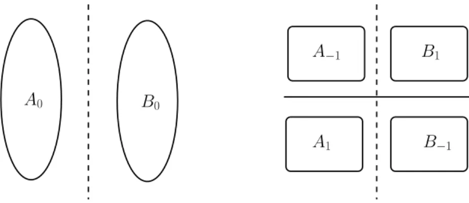
The construction can be followed in Fig. 5.A\A0has been further split intoA1∪A−1:A1is the set of those verticesa withαa = 1 andA−1 is the set of those verticesawith αa =−1; similarly, B\B0 has been further split intoB1∪B−1:B1 is the set of those vertices bwith αb = 1 andB−1 is the set of those verticesb with αb =−1. We haveM1 ⊆(A1×B−1)∪(A−1×B1) since for any edge (a, b) inM, we haveαa+αb =wtM(a, b) = 0.
A
−1A
1B
1B
−1B
0A
0Fig. 5.M0 is the matching M restricted to vertices in A0∪B0 andM1 is the matching M restricted to remaining vertices.
Now we run a transformationM0;Das given in [6]: letG0be the graphGrestricted toA0∪B0. Run Gale-Shapley algorithm in the graphG00 with the starting matchingM00 ={(u+, v−) : (u, v)∈ M0 andu∈A0, v∈B0}, whereG00 is the graph obtained fromG0 as described in Section 2. That is, instead of starting with the empty matching, we start with the matchingM00 inG00; unmatched men inA0propose in decreasing order of preference and whenever a woman receives a proposal from a neighbor that she prefers to her current partner (her preferences as given in G00), she rejects her current partner and accepts this proposal. This results in a stable matching in G00, equivalently, a dominant matchingD in G0, see Section 2. It was moreover shown in [6] that M∗ =M1∪D is a dominant matching inG. We include a new and much simpler proof of this fact below.
Claim 1 The matching M∗=M1∪D is dominant in G.
Proof. The dominant matchingD was obtained as the linear image of a stable matching (call itD0) in G00. LetA01 be the set of a ∈A0 such that (a+, b−)∈D0 for someb ∈B0 and A0−1 =A0\A01. Similarly, letB01be the set ofb∈B0 such that (a−, b+)∈D0 for some a∈A0 andB−10 =B0\B10. See Fig. 6.
A1
A−1 B1
B−1
A0−1 B01
B0−1 A01
Fig. 6.We transformed the stable matchingM0onA0∪B0 to the dominant matchingD: this partitionsA0
intoA01∪A0−1 andB0 intoB10 ∪B0−1. We also haveA\A0=A1∪A−1andB\B0=B1∪B−1.
Observe that every vertex in A01∪B01 is matched inD, however not every vertex inA0−1∪B−10 is necessarily matched inD. That is,A0−1∪B−10 may contain unmatched vertices.
The popular matching M has a witnessα ∈ {0,±1}n: recall that this was the witness used to partition A∪B into A0∪B0 and (A\A0)∪(B\B0). We have αu = 0 for all u∈ A0∪B0 and αu∈ {±1} for allu∈(A\A0)∪(B\B0).
In order to prove the popularity of M∗ = M1∪D, we will show a witness β as follows. For the vertices outside A0∪B0, set βu = αu since nothing has changed for these vertices in the transformationM ;M∗. For the vertices inA0∪B0, setβu= 1 for u∈A01∪B01andβu=−1 for every matched vertexu∈A0−1∪B−10 . For every unmatched vertexu, set βu= 0.
Thusβu≥wtM∗(u, u) for alluandP
u:A∪Bβu= 0: this is becauseD⊆(A01×B−10 )∪(A0−1×B10), so for every edge (a, b)∈D, we haveβa+βb= 0; recall thatαa+αb= 0 for all (a, b)∈M1. What is left to show is thatβa+βb≥wtM∗(a, b) for every edge (a, b).
The correctness of the Gale-Shapley algorithm in G00 to compute popular matchings inG0 im- mediately implies that every edge with both endpoints inA0∪B0 is covered by the sum ofβ-values of its endpoints (see [8]). We will now show that every edge with one endpoint inA0∪B0 and the other endpoint in (A\A0)∪(B\B0) is also covered.
– Every edge inA01×B1is covered sinceβa+βb= 2≥wtM∗(a, b). Similarly every edge inA1×B10 is also covered.
– Consider any edge (a, b)∈A01×B−1. We haveαa= 0 andαb=−1 and sowtM(a, b)≤ −1, i.e., wtM(a, b) =−2 since this is a value in{0,±2}. This means bprefersM(b) =M∗(b) toa. Thus wtM∗(a, b)≤0. Sinceβa = 1 andβb=−1, we haveβa+βb≥wtM∗(a, b). Similarly every edge in A−1×B01is also covered.
– Consider any edge (a, b) inA−1×B−10 . We havewtM(a, b)≤ −1 which means thatwtM(a, b) =
−2. That is, both a and b prefer their partners in M to each other. We will now show that wtM∗(a, b) =−2. SinceM(a) =M∗(a), nothing has changed foraand soaprefersM∗(a) tob.
We claim thatM∗(b)bM(b), i.e.,bis no worse in M∗ than inM.
This is because we ran Gale-Shapley algorithm in G00 with M00 as the starting matching. So if b∈B−10 changed its partner fromu+inM00 tov+inD0thenbprefersvtou. Thus everyb∈B−10 has at least as good a partner in D as in M0. HencewtM∗(a, b) =−2 =βa+βb. By the same reasoning, we can argue that every edge in A1×B−10 is also covered.
– Consider any edge (a, b) inA0−1×B−1. We haveαa = 0 and αb =−1 and sowtM(a, b)≤ −1, i.e., wtM(a, b) =−2. SobprefersM(b) =M∗(b) toa. We claim thatM∗(a)aM(a). This will imply that wtM∗(a, b) =−2.
Recall that D0 is a stable matching inG00: here every vertex prefers outgoing edges to incoming edges, thus every a∈A0−1 gets at least as good a partner asS∗(a) inD, whereS∗ is the men- optimal stable matching in G0; in turn, S∗(a)a M0(a) for all a∈A. HenceM∗(a)a M(a) for everya∈A0−1. ThuswtM∗(a, b) =−2 =βa+βb. We can similarly show that every edge in A0−1×B1 is also covered.
Thus M∗ is a popular matching in G. We will now show that M∗ is a dominant matching inG. Observe thatβu∈ {±1} for every matched vertexu: we will use this fact to show thatM∗ is dominant. Recall thatβu= 0 for all unmatched verticesu. Letρ=ha0, b1, a1, . . . , bk, ak, bk+1ibe any M∗-augmenting path inG. We haveβa0 =βbk+1 = 0, henceβb1 =βak= 1, and soβa1 =βbk=−1.
Either (i) βb2 =−1 or (ii)βb2 = 1 which implies thatβa2=−1. It is now easy to see that in the pathρ, for somei∈ {1, . . . , k−1}the edge (ai, bi+1) has to be labeled (−,−). That is,ρisnotan augmenting path inGM∗. Thus there is noM∗-augmenting path inGM∗, henceM∗ is a dominant
matching inG(by Theorem 2). ut
SinceM is an unstable matching, there is an edge (a, b) that blocksM. SincewtM(a, b) = 2, the endpoints of a blocking edge (a, b) have to satisfyαa =αb = 1; so a∈A1 and b ∈B1. The edge (a, b) blocksM∗ as well since the matchingM1 was unchanged by this transformation ofM0 toD, so M∗(a) =M1(a) andM∗(b) =M1(b), thusaandb prefer each other to their respective partners inM∗. SoM∗ is an unstable dominant matching and Lemma 2 follows.
Lemma 2. IfG,Phas an unstable popular matching thenG,P admits an unstable dominant match- ing.
Hence in order to answer the question of whether every popular matching in Gis stable or not, we need to decide if there exists a dominant matchingM in Gwith a blocking edge. We present a simple combinatorial algorithm for this problem.
Our algorithm is based on the equivalence between dominant matchings inGand stable match- ings inG0. Our task is to determine if there exists a stable matching in G0 that includes a pair of edges (a+, v−) and (u−, b+) such thataandb prefer each other tov andu, respectively, inG. It is easy to decide inO(m3) time whether such a stable matching exists or not inG0.
– For every pair of edgese1= (a, v) ande2= (u, b) inGsuch thataandbprefer each other tov andu, respectively: determine if there is a stable matching inG0 that contains the pair of edges (a+, v−) and (u−, b+).
In the graphG0, we modify Gale-Shapley algorithm so thatbrejects proposals from all neighbors ranked worse than u− and v rejects all proposals from neighbors ranked worse than a+. If the resulting algorithm returns a stable matching that contains the edges (a+, v−) and (u−, b+), then we have the desired matching; else G0 has no stable matching that contains this particular pair of edges.
In order to determine if there exists an unstable dominant matching, we may need to go through all pairs of edges (e1, e2) ∈ E×E. Since we can determine in linear time if there exists a stable matching inG0 with any particular pair of edges [14], the running time of this algorithm isO(m3).
A faster algorithm. It is easy to improve the running time toO(m2). For each (a, b)∈E we check the following.
(◦) Does there exist a stable matching inG0such that (1)a+is matched to a neighbor that is ranked worse than b− in a’s list, and (2) b+ is matched to a neighbor that is ranked worse thana− in b’s list?
We modify the Gale-Shapley algorithm in G0 so that (1) b rejects all offers from superscript + neighbors, i.e., baccepts proposals only from superscript −neighbors, and (2) every neighbor ofa that is ranked better thanb− rejects proposals froma+.
Suppose (◦) holds. Then this modified Gale-Shapley algorithm returns among all such stable matchings, the most men-optimal and women-pessimal one [14]. Thus among all stable matchings that matcha+to a neighbor ranked worse thanb− and that include some edge (∗, b+), the matching returned by the above algorithm matchesbto its least preferred neighbor andato its most preferred neighbor.
Hence if the modified Gale-Shapley algorithm returns a matching that is (i) unstable or (ii) in- cludes an edge (a−,∗) or (iii) matchesb+ to a neighbor better thana−, then there is no dominant matching M in Gsuch that the pair (a, b) blocksM. Else we have the desired stable matching in G0, call this matchingM0.
The projection of the matching M0 on to the edge set ofG will be a dominant matching inG with (a, b) as a blocking edge. Since we may need to go through all edges inE and the time taken for any edge (a, b) isO(m), the entire running time of this algorithm isO(m2). We have thus shown the following theorem.
Theorem 4. Given G= (A∪B, E) on m edges and strict preference lists of its vertices, we can decide in O(m2) time whether every popular matching in Gis stable or not; if not, we can return an unstable popular matching.
4 Finding a non-dominant popular matching
Given an instance G = (A∪B, E),P, the problem we consider here is to decide if every popular matching is also dominant, i.e., to decide if{popular matchings} ={dominant matchings} or not inG.
Problem 2 Input:A bipartite graphG= (A∪B, E)with strict preference lists.
Decide:If there is a non-dominant popular matching in G.
In this section, we show the following.
Theorem 5. Given G = (A∪B, E) with strict preference lists, it is NP-complete to decide if G admits a popular matching that is not dominant.
We start with the following lemma, that is the counterpart of Lemma 2.
Lemma 3. If G,P has a non-dominant popular matching M then G,P admits a non-dominant stable matchingN. IfM is given, then N can be found efficiently.
Proof. LetM be a non-dominant popular matching inGand α∈ {0,±1}n its witness (see Theo- rem 3). We will use the decomposition illustrated in Fig. 5 to show the existence of a non-dominant stable matching inG. As per the decomposition in Fig. 5, M =M0∪· M1. SinceM is not dominant, there exists anM-augmenting pathρinGM (by Theorem 2). The endpoints ofρ(call themuandv) are unmatched inM, henceαu=αv= 0 (see Section 2) and souandv are inA0∪B0.
In the graph GM, the vertices inB−1∪A−1(these vertices have α-value−1) are adjacent only to vertices inA1∪B1 as all other edges incident to vertices inB−1∪A−1 are labeled (−,−), and these are not present inGM. Suppose theM-alternating path ρleaves the vertex setA0∪B0, i.e., suppose it contains a non-matching edge betweenA0∪B0andA1∪B1. Since the partners of vertices in A1∪B1 are in B−1∪A−1, the pathρcan never return toA0∪B0. However we know that the last vertex v of ρis inA0∪B0. Thusρnever leaves A0∪B0, i.e.,ρ is anM0-augmenting path in G∗M
0, whereG∗ is the graphGrestricted to vertices inA0∪B0.
We now run a transformationM1;S as given in [6] to convertM1 into a stable matchingS as follows. The matchingSis obtained by running Gale-Shapley algorithm in the subgraphG1, which is the graphGrestricted to (A\A0)∪(B\B0): however, rather than starting with the empty matching, we start with the matching given byM1∩(A−1×B1). So unmatched men (these are vertices inA1
to begin with) propose in decreasing order of preference and whenever a woman receives a proposal from a neighbor that she prefers to her current partner (her preferences as given inG), she rejects her current partner and accepts this proposal. This results in a stable matchingS inG1.
It was shown in [6] that N =M0∪S is a stable matching in G. We include a new and simple proof of this below (see Claim 2). Sinceρis anM0-augmenting path inG∗M
0 andM0is a subset of N, it follows thatρ is anN-augmenting path inGN. Thus N is a non-dominant stable matching
inG. ut
Claim 2 The matching N=M0∪S is a stable matching in G.
Proof. The matchingS is obtained by running Gale-Shapley algorithm in the graph G1 on vertex set (A\A0)∪(B\B0). We did not compute the matchingS from scratch — we started with edges of the matching M1 restricted to A−1×B1. So in the resulting matching S, it is easy to see the following two useful properties:
– S(b)bM1(b) for everyb∈B1. This is because to begin with, everyb∈B1is matched toM1(b) andbwill change her partner only if she receives a proposal from a neighbor better thanM1(b).
– S(a) a M1(a) for every a ∈ A1. This is because all vertices in B−1 are unmatched in our starting matching and every b∈B−1 prefers her partner in M1 to any neighbor in A−1 (since every edge inA−1×B−1is labeled (−,−) with respect toM1). Thus in the matchingS,awill get accepted either byM1(a) or a better neighbor.
It is now easy to show thatN is a stable matching. We already know thatM0is a stable matching onA0∪B0andS is a stable matching on (A\A0)∪(B\B0). It is left to show that no edge (a, b) with one endpoint in A0∪B0 and another endpoint in (A\A0)∪(B\B0)blocks N, i.e., we need to show thatwtN(a, b)≤0 for every such edge (a, b).
Supposea∈A0 and b∈B−1. Let αbe the witness of M used to partitionA∪B intoA0∪B0
and (A\A0)∪(B\B0). Soαa = 0 andαb =−1, hencewtM(a, b)≤ −1, i.e.,wtM(a, b) =−2. Thus a prefersM0(a) = N(a) to b. Hence wtN(a, b) ≤0. We can similarly show thatwtN(a, b) ≤0 for a∈A−1andb∈B0.
Supposea∈A0 andb∈B1. Then αa = 0 andαb= 1 and sowtM(a, b)≤1, i.e.,wtM(a, b)≤0.
So if a prefers M0(a) = N(a) to b then we can immediately conclude that wtN(a, b) ≤ 0. Else b prefersM1(b) toa and we have noted above that S(b) b M1(b) for everyb ∈ B1. Thusb prefers N(b) =S(b) to aand sowtN(a, b)≤0. We can similarly argue thatwtN(a, b)≤0 for every a∈A1
andb∈B0. This finishes the proof of this claim. ut