Ecological Indicators 85: 853-860. (2018) 1
2
On the reliability of the Elements of Metacommunity Structure framework for separating 3
idealized metacommunity patterns 4
5 6
Dénes Schmera1,2,*, János Podani3,4, Zoltán Botta-Dukát2,5 and Tibor Erős1,2 7
1MTA Centre for Ecological Research, Balaton Limnological Institute, Klebelsberg K. u. 3, H-8392 8
Tihany, Hungary 9
2MTA Centre for Ecological Research, GINOP Sustainable Ecosystem Group, Klebelsberg K. u. 3, H- 10
8392 Tihany, Hungary 11
3Department of Plant Systematics, Ecology and Theoretical Biology, Institute of Biology, L. Eötvös 12
University, Pázmány P. s. 1/c, H-1117 Budapest, Hungary 13
4Ecology Research Group of the Hungarian Academy of Sciences, Budapest, Hungary 14
5MTA Centre for Ecological Research, Institute of Ecology and Botany, Alkotmány u. 2-4, H-2163 15
Vácrátót, Hungary 16
*Correspondence: schmera.denes@okologia.mta.hu 17
18 19
Abstract 20
The Elements of Metacommunity Structure (EMS) framework originally suggested by Leibold 21
and Mikkelson (2002) in Oikos is a popular approach to identify idealized metacommunity 22
patterns (i.e. checkerboard, nested, evenly spaced, Clementsian, Gleasonian), and hereby to 23
infer the existence of structuring processes in metacommunities. Essentially, the EMS 24
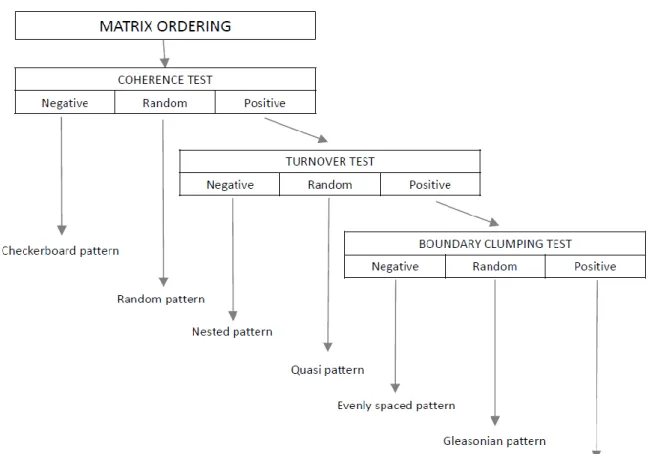
framework consists of the rearrangement of the sites-by-species incidence matrix followed 25
by a series of tests for coherence, turnover and boundary clumping in species distributions.
26
Here, we give a critical evaluation of the EMS framework based on theoretical considerations 27
and simulations. We found that user defined site ordering may influence the coherence test 28
(number of embedded absences) depending also on the ordering of species, and therefore 29
we argue that the application of user-defined matrix rearrangement has strong limitations.
30
The recommended ordering by correspondence analysis is sensitive to matrix structure and 31
may even include arbitrary decisions in special cases. Further, we revealed different 32
meanings of the checkerboard pattern and showed that negative coherence is not 33
necessarily associated with this as assumed in the EMS framework. Also, the turnover test 34
cannot always detect nested pattern, because turnover and nestedness are not necessarily 35
the opposite endpoints of a continuum. We argue that the boundary clumping test can only 36
be used for separating Clementsian, Gleasonian and evenly spaced patterns if sites are 37
ordered along a real environmental gradient rather than a latent one identified by 38
correspondence analysis. We found that the series of tests in the EMS framework are 39
burdened by anomalies and that the detection of some metacommunity patterns is sensitive 40
to type II error. In sum, our findings suggest that the analytical methodology of the EMS 41
framework, as well as the conclusions drawn from its application to metacommunity studies 42
require careful reconsideration.
43 44
Keywords 45
biodiversity; community pattern; pattern analysis; idealized metacommunity patterns 46
47 48
1. Introduction 49
Detecting and understanding drivers of metacommunity structure are key issues in 50
community ecology with significant legacy (Mittelbach 2012). Early ecologists have already 51
inferred the existence of structuring forces from the community patterns observed. For 52
instance, Clements (1916), the pioneer of North American plant ecology, viewed plant 53
communities as coherent units with discrete boundaries formed in response to 54
environmental factors (Clementsian pattern). In contrast, Gleason (1926) argued that species 55
have distinct ecological characteristics and therefore individualistic responses to underlying 56
environmental gradients (Gleasonian pattern). Evenly spaced pattern occurs in systems with 57
trade-offs in fitness in different environments, resulting in a spatial distribution with evenly 58
dispersed populations (Tilman 1982). Intense interspecific competition may generate 59
checkerboard pattern where pairs of species are mutually exclusive (Diamond 1975). Finally, 60
nested pattern occurs when species poor communities consist of subsets of species 61
occurring in richer communities (Patterson and Atmar 1989). These cases have been 62
regarded as idealized types of metacommunity pattern (Ulrich and Gotelli 2013, Heino et al.
63
2015) and have received increasing attention due to their theoretical interpretation 64
(Carvalho et al. 2013, Ulrich and Gotelli 2013).
65
The development of metacommunity theory provided a conceptual framework for ecologists 66
to disentangle underlying drivers (niche based species sorting, dispersal, drift, see Vellend 67
2010, Shipley et al. 2012) of multisite communities (Leibold et al. 2004). Some of the 68
approaches use multispecies distribution patterns for inferring the existence of structuring 69
ecological forces. No doubt that the “elements of metacommunity structure” approach 70
suggested by Leibold and Mikkelson (2002) and its upgrade (Presley et al 2010, hereafter 71
referred to as EMS framework) provide a very popular methodology developed for this 72
purpose.
73
The EMS framework includes the rearrangement of the sites-by-species incidence matrix 74
followed by three tests (Fig. 1), each related to a given element of metacommunity 75
structure. First, the rows and the columns of the matrix are ordered along the first axis of 76
correspondence analysis (CoA) to discern variation in response to a latent environmental 77
gradient. According to Leibold and Mikkelson (2002, p. 241), the simultaneous ordering of 78
sites and species has three purposes: (1) it often minimizes the number of interruptions in 79
species' ranges (number of embedded absences), (2) it provides a basis for judging whether 80
a given metacommunity is nested, or dominated by turnover (high number of species 81
replacements), and (3) it defines the boundaries of species' ranges (boundary clumping).
82
Consequently, matrix rearrangement via CoA has strong impact on the assessment of each 83
element of metacommunity structure. Note that although this procedure is recommended 84
for general use, the EMS framework also allows user-defined matrix ordering. Secondly 85
coherence, the first element of metacommunity structure is defined as the number of 86
embedded absences in the matrix and its significance is examined using null model tests.
87
Following the study of Gotelli (2000), species richness of sites is kept constant in the 88
recommended null model (Presley et al. 2010). If coherence is negative (the number of 89
embedded absences is significantly higher than expected by chance) then the EMS 90
framework detects checkerboard pattern. If the number of embedded absences does not 91
differ significantly from a randomly generated value (coherence is random) then the EMS 92
framework indicates a random pattern. If coherence is positive (the number of embedded 93
absences is lower than expected by chance) then the matrix should be examined for 94
turnover. Turnover, the second element of metacommunity structure, is measured as the 95
number of times one species replaces another between two sites (i.e. number of 96
replacements) for each possible pair of species and for each possible pair of sites. If turnover 97
is negative (the number of replacements is lower than expected by chance) then the EMS 98
framework reveals a nested pattern, if turnover is random the EMS detects quasi pattern 99
(see Presley et al. 2010), and if turnover is positive (the number of replacements is higher 100
than expected by chance) then the EMS framework suggests the existence of Clementsian, 101
Gleasonian or evenly spaced patterns. These latter three are separated from each other by 102
examining the boundary clumping of species ranges, the third element of metacommunity 103
structure, using the Morisita test. If clumping is positive (Morisita I is significantly larger than 104
1.0) then the EMS framework detects Clementsian pattern; if clumping is negative (Morisita I 105
is significantly lower than 1.0) evenly spaced pattern is indicated, and if clumping is random 106
(Morisita I does not significantly differ from 1.0) then the pattern is thought to be 107
Gleasonian.
108
There is, however, much controversy about the relative merits of the EMS framework.
109
Gotelli and Ulrich (2012, p. 178), for instance, noted that species segregation and 110
aggregation examined in the coherence test "might be the different sides of the same coin"
111
and that rearranging the matrix (i.e. the reordering of sites by correspondence analysis) 112
"does not alter any of the underlying information on species occurrences in the matrix". By 113
examining the power of different null model algorithms, Gotelli and Ulrich (2012) found that 114
a segregation measure was not exactly opposite in its behavior to a nestedness measure, 115
suggesting that nested and segregated patterns (i.e. evenly spaced, Gleasonian and 116
Clementsian) are not necessarily mutually exclusive as implied by the turnover test in the 117
EMS framework. The same authors repeated this comment later and also argued that "The 118
frameworks proposed by Leibold and Mikkelson (2002), and Presley et al. (2010) implicitly 119
assume that measures of coherence, turnover, and boundary clumping describe orthogonal, 120
independent properties of matrices. But if the measures are strongly correlated, some of the 121
proposed cells in their classification frameworks may be redundant or not achievable.
122
Leibold and Mikkelson (2002) recognized this problem and noted that they were able to 123
identify empirical matrices that fit each of the five different scenarios they described" (Ulrich 124
and Gotelli 2013, p. 3). A more recent paper stated that the efficiency of the EMS framework 125
is heavily dependent on data quality (Mihaljevic et al. 2015, see also Gotelli and Graves 126
1996, Ulrich and Gotelli 2013) and suggested the use of occupancy models to at least partly 127
overcome this problem. These models allow an estimation of predicted occupancy at each 128
sample site and thus make it possible to distinguish between the probability of a species 129
occurring at a site and the probability of a species being detected at a site in which it does 130
occur (Mihaljevic et al. 2015). These critical comments, however, did not prevent community 131
ecologists from using the methodology even further. The EMS framework has still been used 132
increasingly both in terrestrial and aquatic realms for finding the best fit to idealized 133
metacommunity patterns (Dallas and Presley 2014, de la Sancha 2014, Heino et al. 2015).
134
However, the reliability of the method in discerning idealized (meta)community patterns has 135
not been tested as yet.
136
To fill this methodological gap, this paper examines the performance of the EMS framework.
137
Combining theoretical aspects with simulation approaches we go through this approach step 138
by step and inspect how the rearrangement of the matrix, the output of individual tests as 139
well as their series influence the success of analysis. We examined also the robustness of the 140
methodology to increasing noise in the data, as well as the practice of researchers in 141
revealing the importance of environmental factors structuring metacommunity patterns.
142 143
2. Methods 144
To guarantee unambiguous answers, we first carefully review terms and procedures related 145
to the EMS framework. We discuss possible interpretations of terms and evaluate the 146
performance of different procedures. In case of equivocal use of any term or procedure, we 147
attempt to clarify the situation by suggesting a solution.
148
We calculated the following indices: the number of embedded absences (the index of 149
coherence test, Leibold and Mikkelson 2002, Presley et al. 2010), the number of mutually 150
exclusive species pairs (Diamond 1975), turnover (the index of turnover test, Leibold and 151
Mikkelson 2002, Presley et al. 2010). As nestedness is not defined in the EMS framework, we 152
used two nestedness measures, the relativized nestedness (Nrel, Podani and Schmera 2011) 153
and the site-order independent version of NODF (Almeida-Neto et al. 2008) called as 154
NODFmax (Podani and Schmera 2012, Ulrich and Almeida-Neto 2012).
155
We examined the behavior of indices themselves as well as the behavior of the indices in 156
null model tests. Indices were examined using toy data sets in series of site-by-species 157
incidence matrices. We examined the relationship between indices in two-site situations 158
using the random parameter approach (Chao et al. 2012, see also Baselga and Leprieur 159
2015). In the first (Random parameter approach 1), we assumed that the numbers of species 160
present in both sites (a), present only in the first site (b), and present only in the second site 161
(c) are derived from a uniform distribution ranging from 0 to 100. We generated 50,000 162
triplets of random a, b and c values, and removed data records with empty sites. In the 163
second case (Random parameter approach 2), we assumed that 200 species are distributed 164
among the three sets (a, b and c). We produced all possible combinations and removed data 165
records with empty sites. Furthermore, we simulated all the possible sites-by-species 166
matrices containing 4 sites and 4 species (degenerate matrices were omitted). This 167
procedure resulted in 41,503 binary matrices, called hereafter as 4-by-4 binary matrices.
168
Although the 4-by-4 binary matrices allow examining the response of indices to all possible 169
situations in the matrix, the null model test of the matrix might be problematic due to the 170
small number of sites and species. We therefore produced 10,000 random matrices with 10 171
sites and 10 species (degenerate matrices, i.e. those containing empty rows or columns, 172
were omitted). These are referred to as 10-by-10 matrices. We used them in null model tests 173
(Gotelli and Graves 1996). For each random matrix, we generated 1000 null matrices.
174
Although there are many algorithms to produce 'random' or 'null' matrices and these 175
algorithms have different statistical properties and ecological meanings (Gotelli and Ulrich 176
2012, Ulrich and Gotelli 2013, Strona et al. 2017), we selected the null model method that 177
maintained the species richness of every site and filled species ranges based on their 178
marginal probabilities ("r1" method in metacom package, Dallas 2014). The P value 179
(estimated probability of type I error) was calculated as the number of null matrices whose 180
index value was more extreme than or equal to the observed index. We applied a two-tailed 181
test at = 0.05. The Jaccard index (Jaccard 1912) was used to measure the similarity of 182
different null model tests: the number of matrices proved to be significantly positive (or 183
negative) in both tests was divided by the number of such matrices plus those that were 184
found significant only in either of the two tests. Positive and negative results in the two tests 185
were not distinguished.
186
We used a noise test (Gotelli 2000, Podani and Schmera 2012) to examine the sensitivity of 187
the EMS framework to increasing randomness in community data. We started with 20-by-20 188
perfectly structured nested, Gleasonian, evenly spaced and Clementsian patterns (Electronic 189
Appendix 1). These patterns were regarded as initial patterns (step 0, 0% noise). We then 190
gradually added noise (randomness) to the matrix in the following way: In the first step (5%
191
noise), 20 pairs of randomly chosen values in the matrix were interchanged (referred to the 192
full randomization model in Podani and Schmera 2012). In the second step (10% noise), 40 193
pairs of randomly chosen values were interchanged. Complete randomness (100% noise) is 194
achieved after 20 steps, with a total of 400 interchanges. Degenerate matrices were 195
omitted. This procedure was repeated 100 times for every step. EMS analysis was performed 196
for each step (21 steps) 100 times. The output of the noise test shows the relative frequency 197
of detected metacommunity patterns in response to increasing noise level (from 0% to 198
100%). The ideal - and expected - situation is that at low noise level the methodology detects 199
mostly the initial pattern. At intermediate noise level, the initial pattern is detected in a 200
decreasing number of times, while the frequency of random pattern is increasing. At high 201
noise level, the frequency of random pattern should be the largest. If the initial pattern is 202
not detected many times even at low noise level, then the EMS framework is sensitive to 203
type II error. In contrast, if the initial pattern is detected with high frequency even at high 204
noise level, the EMS framework is sensitive to type I error.
205
Finally, we examined how researchers use the EMS framework and handle the importance of 206
environmental factors in shaping metacommunity patterns. To reveal this, first we made a 207
search using ISI Web of Science (access date: 28 July 2015) on the number of papers citing 208
Presley et al. (2010). In the second step, we searched for papers applying the EMS 209
framework. We divided these papers into two groups: those applying user defined matrix 210
ordering and articles using CoA for site and species ordering. Then, we searched for papers 211
that reported the variance explained by CoA axes. In our view, this information is essential, 212
and should be obligatorily added to EMS analysis as an expression of the reliability of the 213
method. No doubt that the amount of community variation explained must be used for 214
assigning the studied metacommunity to an idealized pattern. Finally, we examined whether 215
the axes of CoA (EMS framework) were related to any environmental variables.
216
All calculations were performed in R (R Core Team 2016). All possible matrices containing 4 217
sites and 4 species were produced by the gtools package (Warnes et al. 2015). Null matrices 218
were produced by the metacom package (Dallas 2014). Correspondence analysis (CoA) was 219
performed by the ca package (Nenadic and Greenacre 2007), the number of mutually 220
exclusive species pairs, number of embedded absences, turnover, relativized nestedness and 221
NODFmax were calculated by R-scripts developed by the authors (Electronic Appendix 2).
222 223
3. Site and species ordering 224
By definition, site and species orderings influence the number of embedded absences 225
(order-dependent measure) in the data matrix, but they have no impact on the number of 226
replacements (order-independent measure). In addition, site ordering also affects patterns 227
in boundary clumping (order-dependent measure). That site and species ordering both 228
influence coherence can be explained by the definition of embedded absence: "an 229
interruption in a range or community" (p. 242 in Leibold and Mikkelson 2002).
230
Studying communities along an environmental gradient is a typical situation for user-defined 231
site-ordering. The EMS framework allows user-defined matrix ordering without emphasizing 232
the importance of species ordering. Since coherence is influenced not only by the order of 233
sites but also by species ordering, as said, user-defined matrix ordering has strong 234
limitations. Therefore, if the data matrix is ordered by the user, we recommend a clear 235
definition of species ordering, if it is possible at all.
236
Alternatively, the recommended matrix-ordering uses the first axis of CoA to define the 237
order of sites (and species) for the coherence test. In this case, we disclaim real 238
environmental gradients and focus on the "within-matrix data structure". In complex data 239
structures, however, the first axis of CoA does not necessarily explain considerably more 240
variation than the subsequent axes. In other words, the first axis of CoA might identify one 241
dominant but not necessarily the only dominant axis of community variation. This means 242
that analyses of the same data matrix reordered along different axes might reveal 243
contrasting aspects of data structure. We by no means state that the use of the first axis of 244
CoA is a bad decision but emphasize that further studies are needed to reveal the effect of 245
choosing among similarly important axes, and to merge alternative results into a consensus.
246
Finally, although CoA has been one of the most popular ordination methods in numerical 247
ecology, it has some limitations. One of these is that sites with single and unique species 248
cannot be ordered due to the lack of overlap with other sites and species. If software 249
packages do order such matrices "in a way" then the result is based on an arbitrary decision 250
(Electronic Appendix 3). Accordingly, CoA performed by different software packages may 251
provide differently ordered matrices and thus it cannot be regarded as "a standardized 252
approach to order sites and species" as stated by Presley et al. (2010, p. 910). Although field 253
ecologists might argue that actual data sets rarely contain sites with unique species, we have 254
three arguments in favor of discussing this situation. First, a methodology should work under 255
all circumstances, or at least its users should be aware of any limitations. Second, the chance 256
of observing sites with unique species cannot be excluded completely in actual data sets.
257
Finally, checkerboard pattern, a key term of the EMS framework, has a strong theoretical 258
connection to sites with unique species (see next paragraph).
259 260
4. The multiple meaning of checkerboard pattern 261
Since the coherence test of the EMS framework is supposed to separate checkerboard, 262
random and other data structures from each other, first we review the meaning of 263
checkerboard pattern and then identify its most conspicuous realization. In examining the 264
co-occurrence of bird species on islands, Diamond (1975) proposed the term "checkerboard 265
distribution" for competing pairs of species with mutually exclusive island-by island 266
distributions. In this metaphor, the distribution of the competing pair of species reflects the 267
alternating squares of dark and light colors in a checkerboard pattern (of which the 268
chessboard is a special case). Accordingly, we can visualize this checkerboard distribution for 269
a given pair of species by the following matrix (M1), where sites are rows and species are 270
columns:
271 272
M1=
1 0
0 1
1 0
0 1 273
274
It is very important to emphasize that Diamond's original checkerboard distribution reflects 275
the distribution of pairs of species, and the "checkerboard character" of a community has 276
been mostly (but not always, see Stone and Roberts 1990, 1992; Gotelli 2000) characterized 277
by the number of checkerboard species pairs (i.e. the number of species pairs with non- 278
overlapping occurrence). In agreement with this, and for compatibility with the EMS 279
framework (Presley et al. 2010), we will use the term checkerboard pattern for binary 280
matrices in which the number of checkerboard species pairs (Stone and Roberts 1990) is 281
high. This definition means that the checkerboard pattern may be identified in binary 282
(presence-absence) matrices without any restriction as to the order of sites and species.
283
Almeida-Neto et al. (2008) used the term "checkerboard" for any binary matrix in which 284
every cell containing the value of 1 has the same value in all diagonally neighboring cells and 285
0 in the remaining neighboring cells, for example:
286 287
M2=
1 0 1 0
0 1 0 1
1 0 1 0
0 1 0 1 288
289
We refer to this as visual checkerboard pattern, which has been used mostly for visualization 290
purposes. Since its first appearance (Almeida-Neto et al. 2008), the visual checkerboard 291
pattern has been used frequently as an example matrix for developing pattern analysis 292
procedures (Podani and Schmera 2011, Ulrich and Gotelli 2013). However, many analytical 293
tools in metacommunity ecology are insensitive to the order of sites and species in the 294
matrix and therefore are unable to detect and test this unique property. A noted example is 295
the compartment pattern, which differs from the visual checkerboard pattern only in the 296
ordering of sites and species (Podani and Schmera 2011, Ulrich and Gotelli 2013).
297
Recently, Connor et al. (2013) have contributed by two very important points to the proper 298
interpretation of the checkerboard pattern in situations where ordering is fixed by 299
geographical constraints. First, they argued that the checkerboard metaphor reflects the 300
mutually exclusive distribution of two species on a set of islands, where only one of the two 301
species (denoted by the letters A or B) is present on a single island, while the position of the 302
letters corresponds to the explicit geographic position of the islands. Consequently, a set of 303
16 islands arranged spatially in a regular 4-by-4 grid and occupied by two species (A and B) 304
shown below indicates a checkerboard pattern:
305 306
A B A B
B A B A
A B A B
B A B A 307
308
Connor et al. (2013) argued also that the metaphor does not intend to visualize the 309
presence-absence of the species in a sites-by-species incidence matrix (for example, M2 as 310
given above) and thus this incidence matrix, in disagreement with other studies (Almeida- 311
Neto et al. 2008, Podani and Schmera 2011, Ulrich and Gotelli 2013), should not be regarded 312
as a "real" spatial checkerboard pattern.
313
As a second contribution, Connor et al. (2013) pointed out that the idea of Diamond's 314
checkerboard distribution includes not only mutually exclusive island-by-island distribution 315
of species pairs, but also the overlapping geographic ranges of the species. According to this 316
argument and without any information on the distribution ranges of species, the lack of co- 317
occurrence due to competition cannot be separated from lack of co-occurrence owing to 318
non-overlapping ranges (spatial turnover). All of these suggest that presence-absence 319
matrices fail to address Diamond's (1975) original idea because a binary data matrix by itself 320
has "no explicit geography" and provides no information on the distribution ranges of 321
species. To clarify the situation, Connor et al. (2013) suggested the term true checkerboard 322
pattern for a pair of species which never co-occur on the same island and the islands 323
occupied by these two species are geographically alternating.
324
In sum, we will use the term checkerboard pattern when the binary matrix contains a large 325
number of checkerboard species pairs. Visual checkerboard pattern refers to a binary matrix, 326
in which zeros regularly alternate with 1-s over columns and rows. Finally, true checkerboard 327
pattern refers to a pair of species which never co-occur on the same island and the islands 328
occupied by these two species geographically alternate.
329
The EMS framework (Presley et al. 2010) refers to Diamond's definition (Diamond 1975), and 330
thus to checkerboard pattern. Some studies using the EMS framework, however, apparently 331
have to do with the visual checkerboard pattern (see Fig. 2 in Tonkin et al. 2017) to which 332
this methodology does not apply.
333
Of the 41,503 4-by-4 binary matrices, the largest number of mutually exclusive species pairs 334
(6) was observed when all sites contained only a unique species (Electronic Appendix 4). This 335
suggests that if the checkerboard pattern is quantified by the number of checkerboard 336
species pairs (as in the EMS framework), then sites with single and unique species will 337
contribute the most to the checkerboard character. Unfortunately, ordering of such matrices 338
is arbitrary in correspondence analysis (Electronic Appendix 3), and thus the application of 339
CoA and exclusive species pairs within the same approach may not be optimal.
340 341
5. Coherence test 342
The first promise of the coherence test is that a high number of embedded absences 343
(negative coherence) indicates checkerboard pattern (high number of checkerboard species 344
pairs). The examination of 4-by-4 binary matrices shows that sites with single and unique 345
species (matrices with the highest number of checkerboard species pairs) have no 346
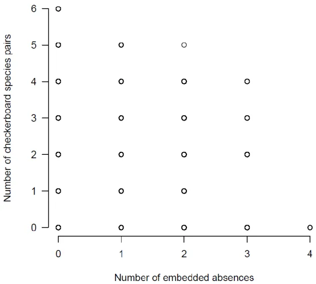
embedded absences. To get a deeper insight into this relationship, we plotted the number of 347
embedded absences (quantifying negative coherence) against the number of checkerboard 348
species pairs (quantifying checkerboard pattern) for the 41,503 4-by-4 incidence matrices 349
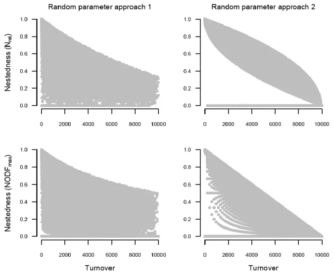
(Fig. 2). As seen, a high number of embedded absences is not necessarily associated with low 350
number of checkerboard species pairs and vice versa. Moreover, 4-by-4 matrices with the 351
highest number of checkerboard species pairs (sites with single and unique species) contain 352
no embedded absences, while matrices with the largest number of embedded absences (not 353
shown) do not contain checkerboard species pairs.
354
The analyses of 10-by-10 matrices revealed that 303 matrices showed a significantly higher 355
number of embedded absences (negative coherence) than expected and thus exhibited 356
checkerboard pattern. The null model test detected 66 matrices with significantly large 357
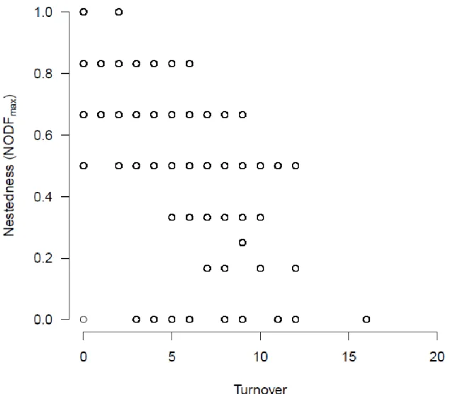
number of checkerboard species pairs, of which 15 matrices were selected also by the 358
coherence test. This suggests that 4.24% (Jaccard similarity = 15/354) is the agreement 359
between null model tests using the number of embedded absences (coherence test of the 360
EMS framework) and the number of checkerboard species pairs. Consequently, the number 361
of embedded absences does not necessarily indicate checkerboard pattern and thus cannot 362
be used alone as its indicator.
363 364
6. Definition of turnover and its test 365
The EMS framework assumes that turnover and nestedness are opposing patterns (Leibold 366
and Mikkelson 2002, p. 239). This means that if we observe low nestedness then turnover 367
should be high and vice versa. In an extreme situation, zero nestedness should yield 368
maximum turnover. To illuminate the relationship between turnover and nestedness, let us 369
examine the following example (rows are sites and species are columns):
370 371
1000000000 372
0111111111 373
374
Here turnover (number of times one species replaces another between two sites: in a two- 375
site situation it means b*c, where b is the number of species present only in the first, while c 376
is the number of species present only in the second site, Presley et al. 2010) equals to 9.
377
Note that in a 2-by-10 incidence matrix the maximum possible value of turnover is 25 378
(obtained when b = 5 and c = 5). Consequently, this turnover value is 64% lower than the 379
theoretical maximum. Although several nestedness indices do exist (the EMS framework 380
does not define any measure), all of them agree that if two sites do not share any species 381
then nestedness should be zero (Ulrich et al. 2009, Podani and Schmera 2012). Thus, this 382
example demonstrates a situation with relatively low turnover and zero nestedness.
383
Before discussing the relationship between turnover and nestedness, we should note that 384
the turnover definition applied by Presley et al. (2010) and used here differs from many 385
existing definitions of turnover (see Tuomisto 2010, Anderson et al. 2011, Gotelli and Ulrich 386
2012). We by no means state that this measure does not quantify the concept of turnover, 387
but emphasize its uniqueness in community ecology and therefore further studies are 388
needed to clarify its performance.
389
We examined the relationship between turnover and nestedness in two-site situations using 390
both random parameter approaches (Fig. 3). All combinations of nestedness measures and 391
random parameter approaches showed that high turnover associates mostly with low 392
nestedness. However, low turnover values can be associated with a wide range of 393
nestedness values, suggesting that turnover and nestedness are not necessarily opposing 394
patterns. Although under specific conditions we can assume that high turnover predicts low 395
nestedness, this is not always the case (see Random parameter approach 2). On the other 396
hand, low turnover does not necessarily predict high nestedness.
397
We studied the relationship between turnover and nestedness using all possible 4-by-4 398
matrices. When nestedness was quantified by the relativized nestedness measure, we found 399
a relatively strong negative relationship between the two variables (r = -0.860, Fig. 4).
400
Although low turnover values indicate high relative nestedness, high turnover does not 401
necessarily indicate low relativized nestedness. When nestedness was quantified by 402
NODFmax, the negative relationship with turnover was lower than with relativized nestedness 403
(r = -0.641, Fig 5), and a low turnover value may be indicative of low nestedness.
404
We used null model tests on 10-by-10 matrices to examine whether significantly high 405
turnover is associated with significantly low nestedness, and whether significantly low 406
turnover with high nestedness. Null model tests indicated 421 matrices with high turnover 407
and 433 matrices with low nestedness when the latter is measured by the relativized 408
measure. The agreement between the two assessments was 23.59% (i.e. Jaccard similarity = 409
163/691). When nestedness was quantified by NODFmax, 296 matrices showed low 410
nestedness. The agreement between high turnover and nestedness (NODFmax) was only 411
5.60% (Jaccard similarity = 38/679). None of our null model tests indicated significantly low 412
turnover, high relativized nestedness and high NODFmax. These results suggest that high 413
turnover is not necessarily associated with low nestedness in the null model tests. In 414
agreement with these findings, Ulrich and Gotelli (2013) and Ulrich et al. (2017) have already 415
published similar results.
416 417
7. Boundary clumping test 418
Our starting point is that Clementsian, Gleasonian and evenly spaced patterns can only be 419
interpreted along an actual (real) environmental gradient (Clements, 1916, Gleason 1926, 420
Tilman 1982, Shipley and Keddy 1987). We argue that "within matrix data structure"
421
revealed by CoA is inadequate for this purpose. Although user defined site ordering might 422
allow testing real environmental gradients, difficulties associated with the coherence test 423
(number of embedded absences is influenced by species ordering, unclear interpretation of 424
coherence) strongly limit this possibility. All of these suggest that no boundary clumping test 425
can be performed within the context of the EMS framework.
426 427
8. Series of tests 428
The EMS framework includes a well-defined sequence of three tests (coherence, turnover 429
and boundary clumping). If we assume that these tests indicate orthogonal and independent 430
properties of matrices then all these tests could be performed independently from the 431
results of tests made earlier in the series. Although Leibold and Mikkelson (2002, p. 239) 432
argue that "turnover and clumping are most meaningful in the context of reasonably 433
coherent ranges", the application of a series of tests has strong consequences. First, a test 434
performed in a series or alone has different statistical and ecological meanings. For instance, 435
the turnover test alone indicates the concept where species are replaced by one another, 436
while within the EMS framework it indicates the existence of replacement in positively 437
coherent metacommunity patterns. Second, some patterns should be more frequently 438
detected than others because earlier tests restrict the possible outputs (i.e. turnover test 439
can only be performed if coherence is high and cannot be performed when coherence is 440
random or negative). Consequently, if we perform a two-tailed statistical test with 5%
441
significance level, then about 2.5% of the examined random matrices should show 442
checkerboard pattern, 95% random pattern, 0.0625% (2.5% × 2.5%) nested pattern, 2.375%
443
(2.5% × 95%) quasi pattern, 0.0015625% (2.5% × 2.5% × 2.5%) evenly spaced and 444
Clementsian pattern, and 0.05937% (2.5% × 2.5% × 95%) Gleasonian pattern in a series of 445
tests suggested by the EMS framework.
446
If we assume that the tests are not orthogonal and not independent then a series of tests 447
may have a clear ecological meaning. In this case, however, the output of an earlier test 448
should predict the output of a later test, or the ecological meaning of the output of an 449
earlier test suggests that there is no need for further ecological information. The argument 450
of Leibold and Mikkelson (2002, p. 239) that "turnover and clumping are most meaningful in 451
the context of reasonably coherent ranges" suggests that the EMS framework considers 452
coherence as primary feature of metacommunity organization. However, we see no strong 453
theoretical support for the priority of coherence in metacommunity structuring.
454 455
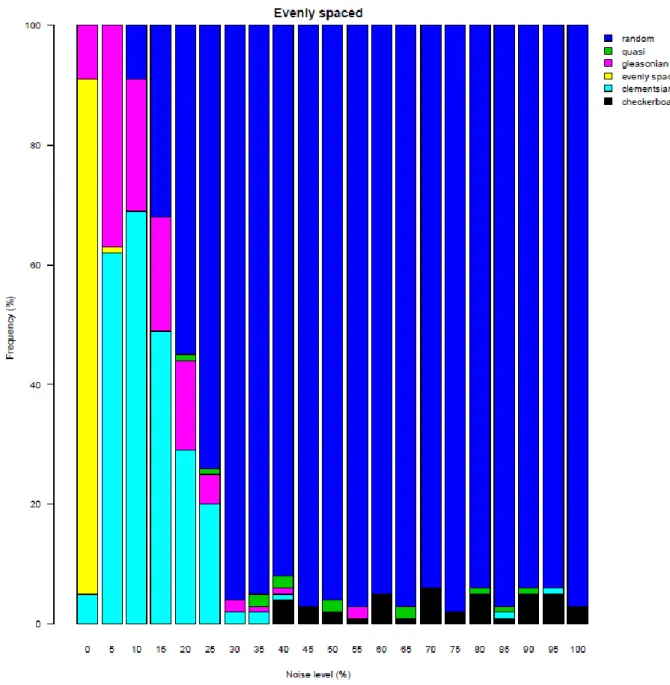
9. Noise test 456
The noise test showed that the reliability of the method to identify idealized structures is 457
different at the same level of noise (Fig. 6, Electronic Appendix 5). For example, the noise 458
level at which the idealized structure was detected at least with 50% reliability was below 459
only 5%, 5%, 10% and 20% for the evenly spaced, Gleasonian, nested and Clementsian 460
gradients, respectively. These results may explain why Clementsian (or quasi-Clementsian) 461
and nested patterns are identified most frequently in actual data sets and why Gleasonian 462
pattern is identified relatively infrequently. Further, identification of the evenly spaced 463
gradient was not possible in all cases even at zero noise. As low as 5% noise in the data 464
already yielded that the EMS method identified either Clementsian or Gleasonian structure.
465
Above 15% (nested), 20% (evenly spaced), 25% (Gleasonian) or 30 % (Clementsian) noise 466
levels, the EMS method identified random metacommunity structure in more than 50% of 467
cases, which further proves the sensitivity of the method to the characterization of idealized 468
structures at different noise levels.
469 470
10. The importance of environmental factors in shaping metacommunity patterns: current 471
practice 472
We found fifty papers citing Presley et al. (2010). Twenty-six papers, each of them ordering 473
sites and species by correspondence analysis, applied the EMS framework. We found that 474
only four papers out of these 26 attempted to provide information on the variance explained 475
by CoA in some way. Three of these 4 papers provided eigenvalues of the first two axes of 476
CoA. However, these two eigenvalues by themselves do not quantify the percentage of 477
variance they explained. There was a single paper of the 26 (3.8%) that provided information 478
on the variance explained by CoA. This paper showed also that the first axis of CoA 479
accounted for 17.7% to 24.0% community variation depending on the metacommunity 480
studied and that environmental variables explained 47.9% to 77.4% variance of the first axis 481
of CoA (Erős et al. 2014). Although this single study does not allow general conclusions to be 482
drawn, it implies that metacommunity patterns are detected based on a limited amount of 483
community variation and that this limited community variation is correlated only at an 484
intermediate-level with multiple environmental variables. In most studies, the variance 485
explained by CoA is not given at all, only the relationship between the site position in 486
ordination axis and environmental variables (80.8%). In some cases, CoA is used in the EMS 487
framework, but environmental variables are related to canonical correspondence analysis by 488
the reasoning that canonical correspondence analysis is related to CoA (de la Sancha et al.
489
2014), or can be regarded as a constrained extension of CoA (Heino et al. 2015). These 490
studies ignore the fact that CoA and canonical correspondence analysis need not result in 491
the same ordering of sites along any ordination axis. Overall, our literature survey shows 492
that essential information, including at least some hints on the reliability of the identification 493
of idealized metacommunity structures remains completely hidden in almost all studies 494
which used the EMS framework.
495 496
11. Conclusions 497
Our theoretical and statistical considerations show that the EMS framework has to be used 498
with caution for the identification of idealized metacommunity patterns. While it is 499
appealing to identify the best-fit metacommunity structure under a single analytical 500
framework, the reliability of the test to distinguish among the idealized structures is strongly 501
case dependent.
502
We showed that although user-defined site-ordering allows testing the response of 503
community to an actual environmental gradient, its application is problematic due to the 504
dependence of the coherence test upon the order of species. Unfortunately, this 505
dependence strongly limits the performance of the EMS framework in testing the response 506
of communities to real environmental gradients. Even if CoA is used for the ordering of sites, 507
the EMS framework is relatively unreliable for separating evenly spaced, Gleasonian and 508
Clementsian patterns. Our results demonstrate that the coherence test is the most critical 509
step of the EMS framework. We found that it is not necessarily adequate for separating 510
checkerboard pattern and its ecological meaning is not clearly defined. Our observations are 511
in strong agreement with the findings of Gotelli and Ulrich (2012) in that the turnover test is 512
not necessarily adequate for detecting a nested pattern.
513
We concluded that the application of a series of tests requires further considerations and 514
that the detection of some idealized patterns is prone to type II error. Our literature survey 515
clearly indicated that the documentation of the results of the EMS framework analysis is 516
insufficient and thus information is extremely limited on the amount of community variation 517
used for detecting idealized metacommunity patterns and also on the relationship between 518
this variation and environmental drivers. These findings call for reconsidering the analytical 519
steps of the EMS framework, and for careful interpretation of its results.
520 521
Acknowledgements 522
523
This work was supported by the OTKA K104279 and the GINOP 2.3.3-15-2016-00019 grants.
524 525 526
References 527
528
Almeida-Neto, M. et al. 2008. A consistent metric for nestedness analysis in ecological systems:
529
reconciling concept and measurement. - Oikos 8: 1227-1239.
530
Baselga, A. and Leprieur, F. 2015. Comparing methods to separate components of beta diversity. - 531
Methods in Ecology and Evolution 6: 1069-1079.
532
Carvalho J.C. et al. 2013. Measuring fractions of beta diversity and their relationships to nestedness:
533
a theoretical and empirical comparison of novel approaches. - Oikos 122: 825-834.
534
Chao, A. et al. 2012. Proposing resolution to debates on diversity partitioning. - Ecology 39: 2037- 535
2051.
536
Clements, F.E. 1916. Plant succession, an analysis of the development of vegetation. Carnegie 537
Institution, Washington.
538
Conor, E.F. et al. 2013. The checker history of checkerboard distributions. - Ecology 94: 2403-2414.
539
Dallas, T. 2014. metacom: an R package for the analysis of metacommunity structure. - Ecography 37:
540
402-405.
541
Dallas, T. and Presley, S.J. 2014. Relative importance of host environment, transmission potential and 542
host phylogeny to the structure of parasite metacommunities. - Oikos 123: 866-875.
543
de la Sancha N.U. et al. 2014. Metacommunity structure in a highly fragmented forest: has 544
deforestation in the Atlantic Forest altered historic biogeographic patterns? - Diversity and 545
Distributions 20: 1058-1070.
546
Diamond, J.M. 1975. Assembly of species communities. In: Cody, M. L. and Diamond, J .D. (eds) 547
Ecology and evolution of communities. Harvard University Press, Boston. pp. 342-444.
548
Erős, T. et al. 2014. Quantifying temporal variability in the metacommunity structure of stream 549
fishes: the influence of non-native species and environmental drivers. - Hydrobiologia 722: 31- 550
43.
551
Gleason, H.A. 1926. The individualistic concept of the plant association. Bulletin of the Torrey 552
Botanical Club 53: 7-26.
553
Gotelli, N.J. 2000. Null model analysis of species co-occurrence patterns. - Ecology 81: 2606-2621.
554
Gotelli, N.J. and Graves, G. 1996. Null models in ecology. Smithsonian Institution Press, Washington, 555
USA 556
Gotelli, N.J. and Ulrich, W. 2012. Statistical challenges in null model analysis. - Oikos 121: 171-180.
557
Heino, J. et al. 2015. Elements of metacommunity structure and community-environment 558
relationships in stream organisms. - Freshwater Biology 60: 973-988.
559
Jaccard, P. 1912. The distribution of the flora in the alpine zone. - New Phytopathologist 11: 37-50.
560
Leibold, M.A. et al. 2004. The metacommunity concept: a framework for multi-scale community 561
ecology. - Ecology Letters 7: 601-613.
562
Leibold, M.A. and Mikkelson, G.M. 2002. Coherence, species turnover, and boundary clumping:
563
elements of meta-community structure. - Oikos 97: 237-250.
564
Mihaljevic, J.R. et al. 2015. Using multispecies occupancy models to improve the characterization and 565
understanding of metacommunity structure. - Ecology 96: 1783-1792.
566
Mittelbach, G.G. 2012. Community Ecology. Sinauer, Massachusetts, USA 567
Nenadic, O. and Greenacre, M. 2007. Correspondence analysis in R, with two- and three-dimensional 568
graphics: The ca package. - Journal of Statistical Software 20: 1-13- 569
Patterson, B.D. and Atmar, W. 1986. Nested subsets and the structure of insular mammalian faunas 570
and archipelagos. - Biol. J. Linn. Soc. 28: 65-82.
571
Podani, J. and Schmera, D. 2011. A new conceptual and methodological framework for exploring and 572
explaining pattern in presence-absence data. - Oikos 120: 1625-1638.
573
Podani, J. and Schmera, D. 2012. A comparative evaluation of pairwise nestedness measures. - 574
Ecography 35: 889-900.
575
Presley, S.J. et al. 2010. A comprehensive framework for the evaluation of metacommunity structure.
576
- Oikos 119: 908-917.
577
R Core Team 2016. R: A language and environment for statistical computing. R Foundation for 578
Statistical Computing, Vienna, Austria (version 3.2.5). URL https://www.R-project.org/
579
Shipley, B. and Keddy, P.A. 1987. The individualistic and community-unit concepts as falsifiable 580
hypotheses. - Vegetatio 69:47–55.
581
Shipley, B. et al. 2012. Quantifying the importance of local niche-based and stochastic processes to 582
tropical tree community assembly. - Ecology 93: 760-769.
583
Stone, L. and Roberts, A. 1990. The checkerboard score and species distributions. - Oecologia 85: 74- 584
79.
585
Stone, L. and Roberts, A. 1992. Competitive exclusion, or species aggregation? - Oecologia 91: 419- 586
424.
587
Strona, G. et al. 2017. Bi-dimensional null model analysis of presence-absence binary matrices. - 588
Ecology (accepted article, doi: 10.1002/ecy.2043) 589
Tilman, D. 1982. Resource competition and community structure. Princeton University Press, 590
Princeton.
591
Tonkin, J.D. et al. 2017. Metacommunity structuring in Himalayan streams over large elevational 592
gradients: the role of dispersal routes and niche characteristics. - Journal of Biogeography 44:
593
62-74.
594
Tuomisto H 2010. A diversity of beta diversities: straightening up a concept gone awry. Part 1.
595
Defining beta diversity as a function of alpha and gamma diversity. Ecography 33: 2-22.
596
Ulrich, W. et al. 2009. A consumer's guide to nestedness analysis. - Oikos 118: 3-17.
597
Ulrich, W. et al. 2017. A comprehensive framework for the study of species co-occurrences, 598
nestedness and turnover. - Oikos 126: 1607-1516.
599
Ulrich, W. and Almeida-Neto, M. 2012. On the meaning of nestedness: back to the basics. - 600
Ecography 35: 865-871.
601
Ulrich, W. and Gotelli, N.J. 2013. Pattern detection in null model analysis. - Oikos 122: 2-18.
602
Vellend, M. 2010. Conceptual synthesis in community ecology. - The Quarterly Review of Biology 85:
603
183-206.
604
Warnes, GR et al. 2015. gtools: Various R programming tools. R package version 3.5.0.
605
https://CRAN.R-project.org/package=gtools 606
607 608
FIGURES 609
610
611
Fig. 1: Diagrammatic representation of the Elements of Metacommunity Structure (EMS) 612
framework following Leibold and Mikkelson (2002) and Presley et al. (2010).
613 614
615
Fig. 2: The relationship of the number of embedded absences and the number of 616
checkerboard species pairs when incidence matrices with 4 sites and 4 species were 617
examined.
618 619
620
Fig. 3: The relationship between turnover (horizontal axes) and nestedness (vertical axes) 621
when pairs of sites were examined. Upper subfigures show when nestedness was quantified 622
as Nrel, while lower subfigures show when nestedness was quantified as NODFmax. Left 623
subfigures show the results of the Random parameter approach 1, while right subfigures 624
those of the Random parameter approach 2.
625 626
627
Fig. 4: The relationship between turnover and nestedness ((Nrel) when incidence matrices 628
with 4 sites and 4 species were examined.
629 630
631
Fig. 5: Relationship between turnover and nestedness (NODFmax) when incidence matrices 632
with 4 sites and 4 species were examined.
633 634
635
Fig. 6: Bar plot showing the frequency of idealized metacommunity patterns (vertical axis) 636
detected by the Elements of Metacommunity Structure (EMS) framework when evenly 637
spaced pattern was exposed to increasing noise (horizontal axis).
638 639 640 641
642
THE MANUSCRIPT CONTAINS ALSO THE FOLLOWING ELECTRONIC APPENDICES 643
644
Electronic Appendix 1: Idealized metacommunity patterns used in the noise test.
645 646
Electronic Appendix 2: R script used for calculating indices.
647 648
Electronic Appendix 3: The ordering of an incidence matrix with sites with single and unique 649
species. R scripts.
650 651
Electronic Appendix 4: Visualization of 4-by-4 incidence matrices with the largest number of 652
checkerboard species pairs.
653 654
Electronic Appendix 5: The results of the noise tests on nested, Gleasonian and Clementsian patterns.
655 656