A distributed quadratic generation scheduling optimization and reserve allocation approach based on the decomposition of generation characteristics

A distributed quadratic generation scheduling optimization and reserve allocation approach based

on the decomposition of generation characteristics

D´avid Csercsik

P´azm´any P´eter Catholic University Faculty of Information Technology P.O. Box 278, H-1444 Budapest

Email: csercsik@itk.ppke.hu

P´eter K´ad´ar

Kand´o K´alm´an Faculty of Electrical Engineering Power System Department - Alternative Energy Technologies

Obuda University B´ecsi ´ut 96/b H-1034 Budapest´ Email: kadar.peter@kvk.uni-obuda.hu

Abstract—The operation with the limited resources requires optimization. Also in an island mode on board energy system or in the large power system the optimal power generation distribution between the operating units is crucial for increase the success of the mission or for the protection of the environment or decrease the costs. A method for generator scheduling and simultaneous allocation of reserves is proposed in this article. Based on the decomposition and piecewise linear approximation of generation characteristics, we formulate the optimization framework in a distributed manner, making the utilization of parallel computing power possible. We define a finite number of operation modes for each generator, and analyze the feasibility and resulting cost of their possible combinations. Secondary and tertiary reserves are also allocated in the process. A simple heuristic is introduced to reduce the number of operating profiles taken into account.

I. INTRODUCTION

It is well known that the market share and significance of renewable technologies in the electric power industry have been largely increased [1], and significant efforts were done to effectively integrate these resources into the existing systems [2], [3]. However, as detailed in [4], the great majority of these renewable resources are variable generators having an availability limit that changes through time and cannot be pre- dicted with perfect accuracy. This variability and uncertainty add to the existing variability and uncertainty of the current systems (eg. uncertain domestic demand), and these additional issues imply unique characteristics and may change the way that system operators maintain a reliable power system.

As long as technically efficient and economically feasible methods for energy storage [5], [6] are not available in industrial scale, the only way to handle these uncertainty issues is the application of system level resources or, in other words, ancillary services [7], [8].

On the other hand, the question how the available power system resources and infrastructure can be utilized in the most economic way is analyzed since the middle of the 20th century [9]. This topic has multiple aspects.

Not only in the power system but also in the aircrafts are several generators. Typically two integrated drive generators supply normally the plane and a third auxiliary generator can

replace either main generator (e.g. in an aircraft A320). In the Boeing 787 the number of the generators are doubled so we count 4 pieces at engine side and 2 more auxiliary units.

The optimal load distribution in normal and emergency case is crucial.

Optimal power flow (OPF) methods aim to optimize the operation of electric power generation, transmission, and dis- tribution networks subject to demand values or functions and transmission and generation system constraints. The literature of OPF is enormous, for recent surveys see [10], [11], [12].

Typical examples when the optimization procedure includes integer variables as well are optimal transmission switching (OTS) and network topology optimization, [13], [14], [15].

The optimal scheduling (OS) of generators, also known as unit commitment (UC) [16] has also a significant size of literature, for surveys see [17], [18], [19]. An integer approach to the problem is described in [20]. Thermal production requirements may be also taken into account [21].

OPF, OTS and OS in general are complex nonlinear large- scale problems. In such cases, decomposition methods [22]

may greatly increase the computational efficiency of solution concepts, even when the price is that only sub-optimal re- sults are obtained. There is a significant amount of results corresponding to the decomposition and decentralization of OPF [23], [24], [25], [26] and OTS in literature. These papers approach the problem by decomposing the computations cor- responding to regions. Such methods receive more and more attention nowadays, as the computing power of parallelized architectures increase [27].

In the terms of OS, the increasing importance of system level resources proposes new challenges and calls for novel solutions. Frameworks which allocate energy production and reserves simultaneously may help reserve-production capable power plants to an increased vindication of their potential: In these frameworks it is immediately taken into account that as they produce energy, they create the potential of reserve allocation as well and in the same time.

In the conference article [28] a model has been introduced in which generation values of generators were optimized over a

set of time intervals in a distributed way implicitly accounting for the requirements of reserve allocation as well. This ap- proach divided the operation range of generators into disjoint sub-regions and assigned modes of operation(MoO) to them.

A MoO profile was defined as a sequence of possible MoOs (a MoO for each time period) for each generator. Considering possible and not possible MoO changes corresponding to consecutive time periods on the one hand and power and reserve demands on the other, a set of top-level feasible MoO profiles may be determined. For each of these top- level feasible MoO profiles, the optimization may be carried out independently (thus in a parallel fashion), considering the availability of the required reserves as set of inequality constraints.

The method proposed in this article assumes that the pro- duction characteristics (in the terms of marginal cost) in each MoO are linearly approximated, and these piecewise linear functions are submitted to the transmission system operator (TSO). Regarding the cost model of this article [28], we have to emphasize that the majority of the corresponding literature (eg. [29]) assumes quadratic total cost, which is usually approximated by piecewise linear functions, implying a linear objective function.

On the other hand, it is widely accepted to assume a constant and a variable component of generation cost. Regarding the variable component, it is plausible to assume that the cost of producing one unit of energy typically has a local minima (at the maximal efficiency point) usually not at maximum capacity.

In this paper we assume two components of the unit cost of generation. First a term corresponding to constant cost, thus described by a term proportional to _x¹ in the context of unit cost, and a quadratic term in the form a+b(x−c)²(wherex denotes the produced quantity). The result of these two terms is a nonlinear, dominantly decreasing function of the produced amount, which we approximate with piecewise linear functions in given intervals (MoOs). This approach, although allows a more realistic consideration of production cost, results in a nonconvex quadratic optimization problem regarding the total cost, thus implying a more difficult computational task.

Start up/shutdown and ramp up/down costs are considered in this approach in the terms of MoO changes: A total cost of a profile in this model depends on

• the exact generation values corresponding to the time periods,

• changeover costs - corresponding to ramp up and ramp down, and start-up -, defined by the MoO profile.

As the variables of the problem are the production or power inlet values, a linear transmission constraint corresponding to a DC load flow model can be easily considered, if the param- eters of the transmission network are known (a demonstrative example shows this issue in the paper [28] ). We assume that the thermal and other technological limitations implying load gradient constraints may be addressed as possible/not possible changes of MoOs in consecutive time periods.

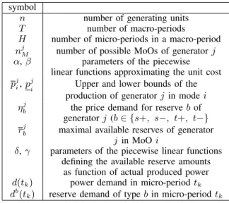
symbol

n number of generating units

T number of macro-periods

H number of micro-periods in a macro-period n^j_M number of possible MoOs of generatorj α,β parameters of the piecewise

linear functions approximating the unit cost p^j_i,p^j

i Upper and lower bounds of the production of generatorj in modei η_b^j the price demand for reservebof

generatorj (b∈ {s+, s−, t+, t−}

r^j_b maximal available reserves of generator jin MoOi

δ,γ parameters of the piecewise linear functions defining the available reserve amounts

as function of actual produced power d(tk) power demand in micro-periodtk

d^b(tk) reserve demand of typebin micro-periodtk

TABLE I PARAMETERS OF THE MODEL

In the current paper, to avoid the computational explosion of integer variables in the case of multiple periods and plants, we extend the concept described in [28] by introducing macro- and micro-periods: Each macro-period is composed of a finite and equal number of micro-periods. MoO changes are allowed only between macro-periods, but power and reserve demands are defined on the level of micro-periods, thus the production values and the values of allocated reserves have to be determined for each micro-period, considering the actual MoO profile.

Furthermore, while the method proposed in [28] only en- sured that the required reserves for each period are available in the case of the MoO profile in question, the method proposed in this article also allocates secondary and tertiary reserves considering the reserve price offered by the generator.

II. THE OPTIMIZATION FRAMEWORK

A. Notations of the model

The notations of parameters and variables of the model are summarized in tables I and II respectively.

s+, s−, t+, t− denote the various types of reserves:

secondary positive, secondary negative, tertiary positive and tertiary negative.

B. Macro- and Micro-periods

We assume that each generator defines for itself a set of finitely manymodes of operation(MoOs), each corresponding to a given interval of the production range. The significance of these MoOs are as follows. We assume that

• For each MoOp^j_i,p^j

i, andr^j_b are defined.

• In any MoO the production cost of one unit of energy and the available reserve production values are approxi- mated by linear functions of the actual production value.

While the real production curve is nonlinear, during the optimization, only the piecewise linear approximations are taken into account. Furthermore, we assume that the

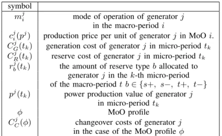
symbol

m^j_i mode of operation of generatorj in the macro-periodi

c^j_i(p^j) production price per unit of generatorjin MoOi.

C_G^j(tk) generation cost of generatorjin micro-periodtk

C_R^j(tk) reserve cost of generator jin micro-periodtk

r^j_b(tk) the amount of reserve typeballocated to generatorjin thek-th micro-period of the macro-periodt b∈ {s+, s−, t+, t−}

p^j(tk) power production value of generatorj in micro-periodtk

φ MoO profile

C_C^j(φ) changeover costs of generatorj in the case of the MoO profile φ

TABLE II VARIABLES OF THE MODEL

difference between the real, nonlinear characteristics and the linear approximation represents the margin of the generator as well (see the appendix for examples).

• When calculating dispatch in consecutive periods, start- up and ramp-up/down costs are considered and reim- bursed to generators based on change of MoOs.

MoOs are assigned to macro-periods, but the power output of generators is calculated for each micro-period. In other words during a certain macro-period, the upper and lower limits of production are fixed for each generator, but within these bounds the particular production values are potentially different for each micro-period in the macro-period.

Macro-periods may be considered as typical daytime load- periods as shoulder or peak load, while micro-periods can be viewed as hours.

In the following the variable t without subscript refers to macro-periods, and with subscript, as t_k, refers to the k-th micro-period of the t-th macro-period (t ∈ [1, ..., T], k∈[1, ...H]).

We assume that for each generator, at anytonly one MoO may be active.

n^j_M

X

i=1

m^j_i(t) = 1 ∀t

An MoO profile φ collects the m^j(t) values as φ_t,j = m^j(t). Furthermore, while formallym^j(t)is a binary vector of sizen^j_m, we also may refer to it shortly. If the generatorjhas 4 MoOs and we saym^j(t) = 3we mean m^j(t) = [0 0 1 0].

In the following we formalize the details of the MoO approach, and define further assumptions of our model.

C. Modeling Assumptions

The modelling assumptions are basically the same as in [28]. We assume that generators provide the parameters about their production characteristics to the transmission system operator (TSO). Linear functions describe the unit cost of production for each MoO as

c^j_i(p^j) =α^j_i+β^j_ip^j (1)

while the total cost may be calculated as a quadratic function of p^j:

C_G^j(tk) =c^j_i(p^j(tk))p^j(tk) (2) The reserve cost may be similarly calculated as

C_R^j(tk) =X

b

ηbr_b^j(tk) (3)

and the maximal reserve to be assigned to a generator is constrained by the inequality (eg. in the case of negative tertiary reserve)

r_t−^j =δ_it−^j +γ_it−^j p^j (4) Regarding the cost of MoO changes, we us suppose that if generatorj changes its MoO fromktol, the changeover cost emerging at the generator, which has to be covered by the TSO is denoted byC_CO^j (k, l). As mode 0 corresponds to shutdown state, these matrices include the start-up costs as well.

Furthermore we assume nonelastic, prior given demand and reserve requirements for each time periodt_k. The objective is to minimize generation cost, including the generators’ margins and reserve costs.

D. The optimization process

The optimization process consists of the following steps

• Based on the initial MoOs, and possible changeovers of the generators, the TSO determines the set of all possible MoO profiles for the given horizon (T macro-periods).

Let us denote a MoO profile byφ

• From the set of possible MoO profiles, the TSO deter- mines the set of the top-level-feasible MoO profiles. Later we detail which constraints limit the set of top-level- feasible MoO profiles.

• The TSO determines thep^j(t_k)andr^j_b(t_k)values for all generators for all top-level-feasible MoO profiles for all tk in a parallel way. In general, it is not sure that all, or moreover any subproblem defined by a particular top- level-feasible MoO profile will be feasible in the terms of the p^j_i(tk) and r^j_b(tk) values, but in this paper we assume that at least one feasible MoO results in a feasible subproblem. As we will see this assumption is supported by the case study.

• The TSO examines the solutions corresponding to the feasible MoOs, and calculates the total cost, which is the sum of the production (or generation) costs (C_G) defined by thep^j_i values resulting from the low level optimization, the reserve costs (CR) implied by ther_b^j(tk)values, and the changeover costsCCO determined by the actual MoO profile.

We call aφprofile feasible, if its top-level-feasible, and also feasible for allt_kin the terms ofp^j(t_k)andr^j_b(t_k). In the final step The total cost of the MoO profileφmay be calculated as C(φ) =CG(φ) +CR(φ) +CCO(φ) (5)

where

C_G(φ) = X

j,t_k

C_G^j(t_k) C_R(φ) =X

j,t_k

C_R^j(t_k)

CCO(φ) = X

j,t,k,l

C_CO^j (k, l)φ(t, j)(k)φ(t+ 1, j)(l) (6)

wherej∈ {1, ..., n},t∈ {1, ..., T −1},k, l∈ {1, ..., n^mj}.

The set of top-level-feasible MoO profiles is restricted by the following considerations:

• Changeover constraints, in other words MoO change restrictions regarding consecutive macro-periods - con- sidering two consecutive t-s, the MoO of any generator may change only by one - eg. no transmission from MoO i toi+ 2 is allowed.

• Possible compulsory standstill and operation period lengths.

• Exclusion of infeasible MoO combinations. If the total power demand at time tk is denoted by d(tk), while the reserve demands are denoted by d^s+(tk), d^s−(tk), d^t+(tk), d^t−(tk). Let us introduce the following notations

d(t) = max

k d(tk) d(t) = min

k d(tk) d^s+(t) = max

k d^s+(tk) d^s−(t) = max

k d^s−(tk) d^t+(t) = max

k d^t+(t_k) d^t−(t) = max

k d^t−(t_k) (7) In this case the following conditions have to be satisfied for the top-level-feasibility of the MoO profile for all t macro-period:

X

i,j

m^j_i(t)p^j

i≤ d(t) ≤X

i,j

m^j_i(t)p^j_i

X

i,j

m^j_i(t)p^j

i≤ d(t) ≤X

i,j

m^j_i(t)p^j_i

d^s+(t)≤X

i,j

m^j_i(t)r^j_is+ , d^s−(t)≤X

i,j

m^j_i(t)r^j_is−

d^t+(t)≤X

i,j

m^j_i(t)r^j_it+ , d^t−(t)≤X

i,j

m^j_i(t)r^j_it−

where the first two rows on inequalities describe that the maximal and minimal demand in a macro-period has to fall between the maximal and minimal possible generation values defined by the MoO, and the rest of the rows correspond to the necessary conditions regarding the feasibility of reserve allocations.

1) The low level optimization process: Considering every top-level-feasible φ,C_G is minimized under the constraints

• Production constraints implied by the MoOs:

p^j

i ≤p^j(t_k)≤p^j_i ∀j, tk (8) where the ivalues are depending on the actual MoO and are straightforwardly determined byφ for eachj andt.

• Reserve constraints: The amount of maximal allocated reserve at tk (r_b^j(tk))is a linear function of the actual production valuep^j(tk)for eachb∈ {s+, s−, t+, t−}.

This linear function is depending on the actual MoO, as described in Table I. and II.

• The total production value has to be equal to the power demand in every micro-period (d(t_k)).

• The total amount of allocated reserves have to meet the demands in every micro-period for all types of reserve (d^s+(t_k), d^s−(t_k), d^t+(t_k), d^t−(t_k)).

As we can see the actual MoO profile implies inequality type constraints, while the power and reserve demands imply equality type constraints. The variable vector to be optimized is

x= xP

xRs

xRt

!

(9) where

xP =

























 p¹(11)

... p¹(1H)

p¹(21) ... p¹(2H)

... pⁿ(TH)



























xRs=































r¹_s+(11) ... rs+¹ (1H)

r¹t+(11) ... r¹t+(1H) rs−¹ (11)

... rs−¹ (1H)





























 xRt=































r¹t−(11) ... r¹t−(1H) r¹_s+(21)

... rt−¹ (TH)

r²_s+(11) ... rt−ⁿ (TH)





























 (10) xP has the dimension nT m, while xR is of dimension 4nT m.

We have to note that since there are negative slope linearities present (in fact, they are dominantly negative sloped), the Q matrix of the quadratic objective function will not be positive definite, thus the problem will not be convex, and solutions may be suboptimal. This drawback is a tradeoff for achiev- ing an efficient, and computationally feasible optimization approach.

III. RESULTS

In this section we demonstrate the operation of the opti- mization framework via the means of an illustrative example, and analyze how the results scale up with the number of macro-periods. We assume 5 generators/power plants whose parameters are described in the Appendix at http://digitus.itk.

ppke.hu/^∼csercsik/SM/appendix.pdf.

A. Heuristic

One of the most challenging problem of the proposed approach is the exponential growth of possible MoO profiles with the increase of the number of macro-periods. A simple heuristic may be introduced to exclude a large portion of the possible profiles.

We may constrain the set of MoO profiles taken into account with the assumption that ifd(t)≤d(t+1) & d(t)≤d(t+1), we consider only MoO profiles in which none of the operation modes decrease as switching fromttot+ 1. In other words, if the minimal and maximal demand are both increased in the next macro-period, we do not allow the down-regulation of

plants in the terms of MoOs. Naturally, we may introduce the complement consideration as well in the case of decreasing maximal and minimal demand.

B. Computational times

We assume the following demands

d(11−46) =[1229 1093 1043 951 1019 1227 1333 1467 1533 1583 1620 1608 1611 1600 1564 1559 1624 1643 1720 1729 1694 1701 1685 1610

Both positive and negative secondary reserve demands are assumed to be equal to 5 % of the power demand for each t_k, and tertiary reserves are assumed being equal to 15 % of the power demand. We assume that the initial MoO profile is [3 3 3 2 2].

The simulations to measure computational demands were run in MATLAB with the OPTI toolbox [30]. The used solver was CLP which has been shown to provide very good results in the case of non-convex quadratic problems [31].

Table III summarizes the performance data of the optimization algorithm on a HP Z440 Workstation Intel Xeon CPU E5-1603 v3 Quad Core processor @ 2.8 GHz, 8 GB.

no parallel computing parallel comput- ing

no. top-level fea- sible profiles

comp. time [s] comp. time [s]

T=2 NH 137 10.38 5.50

H 99 8.38 4.10

T=3 NH 9819 3.504·10³ 1.532·10³

H 1644 611 259

T=4 NH 19614 no data 1.59·10⁵

H 10230 no data 5.36·10³

TABLE III

COMPUTATIONAL PERFORMANCE OF THE OPTIMIZATION FRAMEWORK. NH -NO HEURISTICS, H -HEURISTICS

As we can see in Table III, considering 3 macroperiods, the proposed heuristics and parallel computing together are able to reduce computing time by 1 order of magnitude. Regarding 4 macroperiods, without parallel computing the computations could not be performed (the program crashed), but applying parallel computing and heuristics, the optimization takes about 1.5 hour.

We can see that the more complex cost model and the implied non-convex QP results in computational times much higher compared to a standard MILP approach [32].

IV. DISCUSSION

In this article we presented a decomposition method for the OS problem by the means of introducing MoOs, and a two- level optimization framework. The higher level of the algo- rithm identifies the top-level-feasible MoO profiles considering power and reserve demands and possible production levels determined by the MoO profile. The low level optimization process, which is solved in a parallel way for the top-level- feasible MoO profiles determined by the higher level of the

process, optimizes the power generation and reserve allocation values for each time period according to the constraints defined by the actual profile.

A simple heuristic has been introduced to constrain the number of top-level-feasible MoO profiles taken into account.

The proposed approach may be fit to other, different time scale dispatch algorithms: If any of the PPs has already long term contracts and its generation capacities are partially engaged, it shall submit the piecewise linear approximation only regarding its remaining capacities to the TSO. In this case its number of possible operation modes (n^j_M) may also be decreased, since no shut-down mode is needed, which also decreases the number of possible MoO profiles.

We demonstrated the functioning of the algorithm on a sim- ple example (T=2), and analyzed its performance in the case of larger problems (T=3,4), and compared the computational performance with or without parallel computations and heuris- tics. The results clearly show that the proposed method is able to exploit the capabilities of the available parallel computing power to significantly decrease computational times.

The higher level of the optimization procedure, where MoOs are assigned to generators for each time step, is however tangible for intuition and thus gives space for further heuristic approaches. A possible approach for handling the complexity problems may be the application of suboptimal solutions. If the amount of top-level-feasible MoO profiles largely exceeds the amount which can be efficiently handled, it may do matter which MoO profiles are evaluated first. If eg. a total cost limit is given under which the operation has to be ensured, not all MoO profiles must be evaluated (if a suitable one is found, the algorithm may stop).

The other benefit of the integer approach of the top level procedure is that the MoO profiles may easily combined with other discrete variables, as transformer tap settings or FACTS states, which represent additional control input to the system. Discrete variables corresponding to network topology optimization may be integrated in the same way.

We have to note furthermore that although in the defined framework ramp-up costs are only considered in the terms of MoO changes, this assumption may be easily relaxed. Once the production values for a given MoO profile are determined by the low-level optimization, these costs may be calculated and taken into account during the determination of the total cost of the given MoO profile.

V. ACKNOWLEDGMENTS

This work was supported by grant PD 123900 of the Hungarian National Research, Development and Innovation Office, and by Fund KAP18-1.1-ITK of the P´azm´any P´eter Catholic University.

VI. REFERENCES

REFERENCES

[1] J. Twidell and T. Weir,Renewable energy resources. Routledge, 2015.

[2] J. C. Smith, M. R. Milligan, E. A. DeMeo, and B. Parsons, “Utility wind integration and operating impact state of the art,”IEEE transactions on power systems, vol. 22, no. 3, pp. 900–908, 2007.

[3] E. Ela, M. Milligan, B. Parsons, D. Lew, and D. Corbus, “The evolution of wind power integration studies: past, present, and future,” inPower

& Energy Society General Meeting, 2009. PES’09. IEEE. IEEE, 2009, pp. 1–8.

[4] E. Ela, B. Kirby, N. Navid, and J. C. Smith, “Effective ancillary services market designs on high wind power penetration systems,” inPower and Energy Society General Meeting, 2012 IEEE. IEEE, 2012, pp. 1–8.

[5] H. Chen, T. N. Cong, W. Yang, C. Tan, Y. Li, and Y. Ding, “Progress in electrical energy storage system: A critical review,”Progress in Natural Science, vol. 19, no. 3, pp. 291–312, 2009.

[6] K. Bradbury, “Energy storage technology review,”Duke University, pp.

1–34, 2010.

[7] Y. G. Rebours, D. S. Kirschen, M. Trotignon, and S. Rossignol,

“A survey of frequency and voltage control ancillary servicespart i:

Technical features,”IEEE Transactions on power systems, vol. 22, no. 1, pp. 350–357, 2007.

[8] ——, “A survey of frequency and voltage control ancillary servicespart ii: Economic features,”IEEE Transactions on power systems, vol. 22, no. 1, pp. 358–366, 2007.

[9] C. Baldwin, K. Dale, and R. Dittrich, “A study of the economic shutdown of generating units in daily dispatch,”Transactions of the American Institute of Electrical Engineers. Part III: Power Apparatus and Systems, vol. 78, no. 4, pp. 1272–1282, 1959.

[10] K. Pandya and S. Joshi, “A survey of optimal power flow methods,”

Journal of Theoretical & Applied Information Technology, vol. 4, no. 5, 2008.

[11] S. Frank, I. Steponavice, and S. Rebennack, “Optimal power flow: a bibliographic survey i,”Energy Systems, vol. 3, no. 3, pp. 221–258, 2012.

[12] ——, “Optimal power flow: a bibliographic survey ii,”Energy Systems, vol. 3, no. 3, pp. 259–289, 2012.

[13] E. B. Fisher, R. P. O’Neill, and M. C. Ferris, “Optimal transmission switching,”Power Systems, IEEE Transactions on, vol. 23, no. 3, pp.

1346–1355, 2008.

[14] K. W. Hedman, S. S. Oren, and R. P. O’Neill, “A review of transmission switching and network topology optimization,” in Power and Energy Society General Meeting, 2011 IEEE. IEEE, 2011, pp. 1–7.

[15] K. W. Hedman, R. P. O’Neill, E. B. Fisher, and S. S. Oren, “Optimal transmission switching with contingency analysis,”Power Systems, IEEE Transactions on, vol. 24, no. 3, pp. 1577–1586, 2009.

[16] N. P. Padhy, “Unit commitment-a bibliographical survey,”IEEE Trans- actions on power systems, vol. 19, no. 2, pp. 1196–1205, 2004.

[17] B. H. Chowdhury and S. Rahman, “A review of recent advances in economic dispatch,” 1990.

[18] H. Y. Yamin, “Review on methods of generation scheduling in electric power systems,”Electric Power Systems Research, vol. 69, no. 2, pp.

227–248, 2004.

[19] X. Xia and A. Elaiw, “Optimal dynamic economic dispatch of gener- ation: a review,”Electric Power Systems Research, vol. 80, no. 8, pp.

975–986, 2010.

[20] A. I. Cohen and M. Yoshimura, “A branch-and-bound algorithm for unit commitment,”IEEE Transactions on Power Apparatus and Systems, no. 2, pp. 444–451, 1983.

[21] S. Sen and D. Kothari, “Optimal thermal generating unit commitment:

a review,”International Journal of Electrical Power & Energy Systems, vol. 20, no. 7, pp. 443–451, 1998.

[22] A. J. Conejo, E. Castillo, R. Minguez, and R. Garcia-Bertrand, De- composition techniques in mathematical programming: engineering and science applications. Springer Science & Business Media, 2006.

[23] A. J. Conejo and J. A. Aguado, “Multi-area coordinated decentralized dc optimal power flow,”Power Systems, IEEE Transactions on, vol. 13, no. 4, pp. 1272–1278, 1998.

[24] A. G. Bakirtzis and P. N. Biskas, “A decentralized solution to the dc-opf of interconnected power systems,” Power Systems, IEEE Transactions on, vol. 18, no. 3, pp. 1007–1013, 2003.

[25] P. N. Biskas, A. G. Bakirtzis, N. I. Macheras, and N. K. Pasialis, “A decentralized implementation of dc optimal power flow on a network of computers,”Power Systems, IEEE Transactions on, vol. 20, no. 1, pp.

25–33, 2005.

[26] T. Erseghe, “Distributed optimal power flow using admm,” Power Systems, IEEE Transactions on, vol. 29, no. 5, pp. 2370–2380, 2014.

[27] J. Nickolls, I. Buck, M. Garland, and K. Skadron, “Scalable parallel programming with cuda,”Queue, vol. 6, no. 2, pp. 40–53, 2008.

[28] D. Csercsik and P. K´ad´ar, “A distributed optimal power flow approach based on the decomposition of generation characteristics,” inEnviron- ment and Electrical Engineering (EEEIC), 2016 IEEE 16th International Conference on. IEEE, 2016, pp. 1–6.

[29] M. Carri´on and J. M. Arroyo, “A computationally efficient mixed-integer linear formulation for the thermal unit commitment problem,” IEEE Transactions on power systems, vol. 21, no. 3, pp. 1371–1378, 2006.

[30] J. Currie and D. I. Wilson, “OPTI: Lowering the Barrier Between Open Source Optimizers and the Industrial MATLAB User,” inFoundations of Computer-Aided Process Operations, N. Sahinidis and J. Pinto, Eds., Savannah, Georgia, USA, 8–11 January 2012.

[31] D. Csercsik and P. K´ad´ar, “Performance analysis of matlab solvers in the case of a quadratic programming generation scheduling optimization problem,” inProceedings of the 19th International Conference on Power Electronics and Power Systems, 2017, pp. 3485–3489.

[32] B. F. Hobbs, M. H. Rothkopf, R. P. O’Neill, and H.-p. Chao,The next generation of electric power unit commitment models. Springer Science

& Business Media, 2006, vol. 36.