MŰHELYTANULMÁNYOK DISCUSSION PAPERS
INSTITUTE OF ECONOMICS, CENTRE FOR ECONOMIC AND REGIONAL STUDIES, HUNGARIAN ACADEMY OF SCIENCES - BUDAPEST, 2019
MT-DP – 2019/1
Gender differences in risk aversion and patience:
evidence from a representative survey
DÁNIEL HORN – HUBERT JÁNOS KISS
Discussion papers MT-DP – 2019/1
Institute of Economics, Centre for Economic and Regional Studies, Hungarian Academy of Sciences
KTI/IE Discussion Papers are circulated to promote discussion and provoque comments.
Any references to discussion papers should clearly state that the paper is preliminary.
Materials published in this series may subject to further publication.
Gender differences in risk aversion and patience:
evidence from a representative survey
Authors:
Dániel Horn senior research fellow
Institute of Economics, Centre for Economic and Regional Studies, Hungarian Academy of Sciences and Eötvös Loránd University
email: horn.daniel@krtk.mta.hu
Hubert János Kiss senior research fellow
Institute of Economics, Centre for Economic and Regional Studies, Hungarian Academy of Sciences and Eötvös Loránd University
email: kiss.hubert.janos@krtk.mta.hu
January 2019
Gender differences in risk aversion and patience:
evidence from a representative survey
Dániel Horn – Hubert János Kiss
Abstract
We measure risk aversion and patience in a non-incentivized way using a representative sample of the Hungarian adult population. We elicit risk aversion with a task similar to Gneezy and Potters (1997)'s investment game and find that females risk about 8.5 % less than males when we do not consider any additional controls. However, even when we add extensive controls (related to demography, region, family, education, employment, income and wealth) the difference decreases only slightly and remains significant at conventional levels. We carry out the same exercise for patience and document no significant gender differences in any specification.
Keywords: gender differences, patience, representative survey, risk attitude JEL classification: D8; J16
Nemi különbségek kockázatkerülésben és türelemben:
tanulságok egy reprezentatív felmérésből
Horn Dániel – Kiss Hubert János
Összefoglaló
A magyar felnőtt lakosság reprezentatív mintáján mérjük a kockázatkerülést és a türelmet nem ösztönzött módon. A kockázatkerülést Gneezy és Potters (1997) befektetési játékához hasonló feladattal ragadjuk meg és azt találjuk, hogy a nők megközelítőleg 8,5 százalékkal kisebb összeget kockáztatnak, mint a férfiak, ha nem veszünk figyelembe egyéb tényezőket.
Amikor számos (demográfiához, régióhoz, családhoz, végzettséghez, munkavállaláshoz, jövedelemhez és vagyonhoz kapcsolódó) kontrollváltozót is felhasználunk, akkor az előző különbség csupán enyhén csökken és a szokásos szignifikanciaszintek mellett is jelentős marad. A türelemmel kapcsolatos nemi különbségeket ugyanilyen módon vizsgáljuk, de semmilyen specifikációban nem találunk szignifikáns különbségeket.
Kulcsszavak: kockázatkerülés, nemi különbségek, reprezentatív felmérés, türelem
JEL kódok: D8; J16
Gender differences in risk aversion and patience:
evidence from a representative survey
Horn D´aniel ´es Kiss Hubert J´anosa,b
aMTA KRTK KTI and E¨otv¨os Lor´and University
1097 Budapest, T´oth K´alm´an u. 4. and 1117 Budapest, P´azm´any s´et´any 1/a, Hungary.
e-mail:horn.daniel@krtk.mta.hu
bMTA KRTK KTI and E¨otv¨os Lor´and University
1097 Budapest, T´oth K´alm´an u. 4. and 1117 Budapest, P´azm´any s´et´any 1/a, Hungary.
e-mail:kiss.hubert.janos@krtk.mta.hu
Abstract
We measure risk aversion and patience in a non-incentivized way using a rep- resentative sample of the Hungarian adult population. We elicit risk aversion with a task similar to Gneezy and Potters (1997)’s investment game and find that females risk about 8.5 % less than males when we do not consider any additional controls. However, even when we add extensive controls (related to demography, region, family, education, employment, income and wealth) the difference decreases only slightly and remains significant at conventional levels. We carry out the same exercise for patience and document no signifi- cant gender differences in any specification.
Keywords: Gender differences, patience, representative survey, risk attitude
JEL codes: D8; J16
1. Introduction
The last decades have seen an increasing interest in gender differences in preferences. Surveys (see Croson and Gneezy, 2009; Bertrand, 2011; Niederle, 2016, and references therein) indicate a significant gender difference in com- petitive differences (males being more competitive) and risk aversion (females being more risk averse), though this last result depends on the elicitation method (see Niederle, 2016, for details). The cited surveys find mixed re- sults for social preferences. Interestingly, less is known on gender differences
Preprint submitted to Elsevier January 11, 2019
in time preferences. For instance, none of the previous surveys investigates this issue and the existing results are mixed.1
We contribute to the literature by analyzing gender differences in risk and time preferences based on a survey that is representative of the adult popu- lation of Hungary and that allows the use of a wide array of controls. Our contribution is twofold. On the one hand, most of the evidence on gender differences is based on lab experiments, with a generally non-representative sample of the population (mainly students). Findings on risk attitude from a representative study furthers our understanding on gender differences in preferences. On the other hand, there is still no consensus on whether there is a gender difference in time preferences, thus our finding represents a con- tribution to this debate.
Falk et al. (2018) use representative samples from 76 countries and also study gender differences in preferences. After controlling for country and subnational region fixed effects, they report that women are substantially (by about 20% of a standard deviation) more risk averse than men. Moreover, in 95% of countries, women exhibit greater risk aversion, the difference being at least marginally significant in 82% of the cases. Regarding patience, women are less patient than men, but the difference is small. When investigating gender differences in patience on country level, in only about two-third of the countries do the coefficients reveal a greater degree of impatience for women, and the difference is significant (at least at 10%) in only 32% of the countries. Our study complements (Falk et al., 2018) in the following ways.
We use an extensive set of controls and are able to assess if gender differences persist when taking into account a wide array of variables. Moreover, our risk measurement differs from Falk et al. (2018).
Dohmen et al. (2011) use - among other data sources - a representative German sample. They show that gender is an important determinant of self- assessed risk attitude and they also find that answers to such self-assessed survey correlate strongly with choices in an incentivized experiment on risk attitude, lending support to the view that unincentivized, but large and representative surveys are a useful source of information. The study reports a strong gender difference in the self-assessed risk attitude, female being more risk averse.
1For instance, Dittrich and Leipold (2014) report that males are more impatient while Wang et al. (2016) document no gender differences.
We find a significant gender difference in risk aversion (elicited through a game resembling the investment game by Gneezy and Potters (1997)) even after controlling for age, ethnicity, region, settlement type, marital status, number of children, educational attainment, income, wealth, financial diffi- culties, and employment type and status. However, we do not see any sig- nificant gender difference in patience in any specification that we consider.
2. Data and preference measurement
A survey with a sample size of about 1000 individuals aged 18+ is car- ried out on a quarterly basis by the T ´ARKI Social Research Institute. The survey is based on personal interviews, applies random selection sampling, and is representative of the Hungarian adult population in terms of gender, age, educational attainment and settlement type. The survey has a fixed part, including very extensive data on gender, age, family status and struc- ture, level of education, labour market status, individual and family incomes, wealth and financial situation, social status, religiosity. Researchers can add questions to the survey at a cost.
We introduced questions into the survey of January, 2017. We measured risk aversion with a simple question, asking how much of 10000 Forints the individual would place as a bet in a gamble.2 A bag contained 10 black and 10 red balls and one was drawn randomly. The individual could choose a colour (black or red) and if the colour of the ball drawn coincided with her chosen colour, then she won the double of the bet she placed. If the colour of the ball drawn from the bag was different from the chosen colour, then the bet was lost. We explained also that the amount not placed as a bet would be given to the individual. We regard the amount placed as bet as a natural measure of risk attitude. Our measure is very similar to the investment game of Gneezy and Potters (1997).3
We measured time preferences with 5 questions aiming at finding the approximate indifference point between an earlier and a later amount of money. Similarly to Falk et al. (2018) we used interdependent hypothetical binary choices between 10000 Forints (about 32.26 EUR / 34.48 USD) today
2For details, see section Appendix A in the Supplementary material.
3Charness and Gneezy (2012) report that out of 15 experimental papers using the investment game 14 find a significant gender difference in risk taking, females being more risk averse.
3
or X Forints in a month. The 10000 Forints remained constant during the 5 questions while the amount X was changed systematically depending on the previous answers. For instance, if an individual preferred 10000 Forints today to X=15500 Forints in a month, then it indicated that her indifference point is higher than 15500 Forints, hence in the next question X was increased. 4 Falk et al. (2016) show that this method is a valid measure of time preferences.
The difference between the future X Forints and the current 10000 Ft is a measure of patience as it expresses how much money is needed to compensate the respondent for having to wait a month. The larger is this amount, the more impatient an individual is.5
Similarly to Falk et al. (2018), we did not incentivize the tasks.
3. Results
We present our results using coefficient plots. The coefficient plots visu- alize the estimation of the coefficient with the corresponding standard errors.
We relegate the corresponding OLS regression outputs to section Appendix B in the Supplementary material.
We estimate various models. The graphs show the female coefficient, or in other words the female - male differences in risk aversion and in patience.
In the first model we have no additional controls reflecting the raw gender differences. Then, in later models we add more and more controls. The second specification has a set of controls that we term exogeneous: age, age squared and if the interviewer believes that the respondent is of Roma ori- gin.6 The next set of control variables called region includes dummies for the NUTS3 regions of Hungary and the type of settlement the respondent lives in. The fourth set of control variables are related to family and contains dummies related to the marital status (single, married, separated, living with partner, widow, divorced) and the number of children of the respondent. We have also control variables associated with education including dummies if
4Section Appendix A in the Supplementary material contains the whole structure of the elicitation with the numbers that we used.
5We carried out this time preference elicitation on the 0 vs. 1 month and on the 12 vs. 13 months horizon. Pairwise correlation between choices on the 0-1 and the 12-13 months time horizon is 0.66, significant at even 0.001%. This indicates consistency: those respondents that are more patient on the shorter horizon, tend to be more patient on the longer horizon as well.
6It is forbidden by law to ask directly about ethnicity.
the respondent has a higher than basic education and if the respondent has a tertiary education degree. The set of control variables related to income contain information on the income level, on the wealth level (measured by owning different durables and real estate) and on financial difficulties (hav- ing experienced problems paying utility bills or repaying mortgages or other outstanding loans). The last set of control variables is related to employment and has information on if the respondent works in the private / public sector and her labour market status (e.g. unemployed, employee, employed, inac- tive etc.). The sequence in which we presented our sets of control variables reflects the order as we include them in the regressions. Each new regression adds a new set of control variables to the ones that appeared in the previous regressions.
−15−10−50%
female
no other control +exogeneous
+region +family
+education +income +employment
Figure 1: Female-male differences in risk aversion
In Figure 1, on the vertical axis we depict the percentage difference in the amount that females and males risked in the hypothetical gamble. Negative values indicate that females risked a lower share of their endowment in the gamble. We observe that the difference is significant at 5%-level even if we control for a host of variables, while the gap decreases only slightly from 8.7%
to 6%. This is evidence of a strong gender difference in risk taking using a representative sample and controling for a wide array of variables.
5
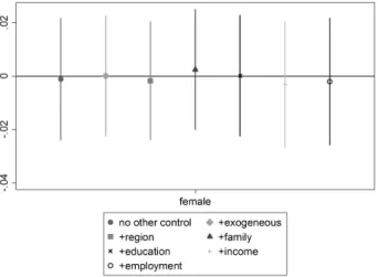
Figure 2 follows the same logic as Figure 1. The vertical axis represents the percentage gender difference in the amount of money needed to com- pensate for having to wait a month.7 We do not see any significant gender difference in any of the specifications.
Figure 2: Female-male differences in patience
4. Conclusion
This study contributes to the literature on gender differences in prefer- ences based on representative samples. In line with the experimental liter- ature using the Gneezy and Potters (1997)’s investment game and findings in Falk et al. (2018) based on representative samples from 76 countries we also document that women are significantly more risk averse than men, even if we take into account a wide range of controls. Regarding patience, we do not find any gender differences.
7That is, the average difference in the amounts needed to compensate is divided by 10000.
5. Acknowledgements
This research was supported by the Higher Education Institutional Excel- lence Program of the Ministry of Human Capacities in the framework of the
’Financial and Public Services’ research project (1783-3/2018/FEKUTSTRAT) at Corvinus University of Budapest. We also acknowledge support from the National Research, Development & Innovation (NKFIH) project K124396.
Hubert J. Kiss thanks support from the NKFIH project K119683.
7
Bertrand, M., 2011. New perspectives on gender. In: Handbook of Labor Economics. Vol. 4. Elsevier, pp. 1543–1590.
Charness, G., Gneezy, U., 2012. Strong evidence for gender differences in risk taking. Journal of Economic Behavior & Organization 83 (1), 50–58.
Croson, R., Gneezy, U., 2009. Gender differences in preferences. Journal of Economic literature 47 (2), 448–74.
Dittrich, M., Leipold, K., 2014. Gender differences in time preferences. Eco- nomics Letters 122 (3), 413–415.
Dohmen, T., Falk, A., Huffman, D., Sunde, U., Schupp, J., Wagner, G. G., 2011. Individual risk attitudes: Measurement, determinants, and behav- ioral consequences. Journal of the European Economic Association 9 (3), 522–550.
Falk, A., Becker, A., Dohmen, T., Enke, B., Huffman, D., Sunde, U., 2018.
Global evidence on economic preferences. The Quarterly Journal of Eco- nomics 133 (4), 1645–1692.
Falk, A., Becker, A., Dohmen, T., Huffman, D. B., Sunde, U., Jan. 2016. The Preference Survey Module: A Validated Instrument for Measuring Risk, Time, and Social Preferences. IZA Discussion Papers 9674, Institute for the Study of Labor (IZA).
URL https://ideas.repec.org/p/iza/izadps/dp9674.html
Gneezy, U., Potters, J., 1997. An experiment on risk taking and evaluation periods. The Quarterly Journal of Economics 112 (2), 631–645.
Niederle, M., 2016. Gender. In: Handbook of Experimental Economics.
Vol. 2. Princeton University Press, pp. 481–553.
Wang, M., Rieger, M., Hens, T., 2016. How time preferences differ: Evidence from 53 countries. Journal of Economic Psychology 52, 115–135.
Appendix A. Supplementary material - Survey questions
1. During the next questions we will play a short game. You have to choose between two amounts of money. Not only are the amounts different, they also differ in when you would receive them. Please assume there is no inflation, i.e., future prices are the same as today’s prices. This situation is hypothetical, but please answer as if it was a real choice.
1.a. Would you rather receive 10000 Forints today or X1 in a month?
1 – 10,000 Ft today, or 2 – X1 Ft in a month?
9 – Do not know
(And 4 other questions of this sort followed.)
2. Please assume that you receive 10000 Forints and you have the op- portunity to place a bet (between 0 and 10000 Ft) on a colour in the next gamble. There is a bag that contains 10 black and 10 red balls. We will draw one. If the colour of the ball drawn coincides with your bet, then we double the amount of your bet. If not, the your bet is lost. The amount not placed as bet is yours.
Please, select a colour!
2.a Selected colour:
2.b. How much would you bet?
Amount of the bet:
3. Now I will ask similar questions as before, but there is a differ- ence. You would receive the earlier payoff in a year, and the later payoff in a year and a month. How would you choose?
3.a. Would you rather receive 10000 Forints in a year or X1 in a year and a month?
1 – 10,000 Ft today, or 2 – X1 Ft in a month?
9 – DK
(And 4 other questions of this sort followed.)
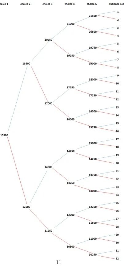
The staircase method is represented in Figure A.3. First, we asked if the individual preferred 10000 Forints today or 15500 Forints in a month. The choice of the former / latter one revealed that the amount of money in a month that makes the respondent indifferent to 10000 Forints today is more / less than 15500 Forints, therefore the next choice involved 10000 Forints
9
today or 18500 / 12500 Forints in a month. We repeated this algorithm in all the 5 questions.
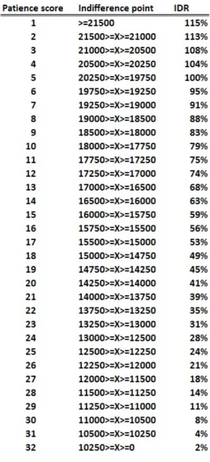
Figure A.4 shows the patience scores and the corresponding upper and lower bounds of the indifference point.
We consider the midpoint of the bounds to compute the individual dis- count rate (IDR). If we denote the midpoint by X, then
(1 +IDR)∗10000 =X, (A.1)
and therefore
IDR= (X/10000)−1. (A.2)
The corresponding individual discount rates are shown in the last column of Figure A.4.
Figure A.3: Tree for the staircase time preference task
11
Figure A.4: Patience scores, the corresponding upper and lower bounds of the indifference point and the implied individual discount rates
Appendix B. Supplementary material - OLS regressions
This section contains the regressions related to risk aversion and patience.
Here we present the complete regression outputs of the different specifica- tions.
The female dummy captures the difference is risk attitudes as the dif- ference in the amount that the individuals placed as a bet. Age and age2 indicates the effects related to age. Roma is a dummy with value of 1 if the interviewer believes that the respondent is of Roma origin. These variables are called exogeneous in Figure 1.
The next set of variables are termedregion. These include six dummies for the NUTS3 regions of Hungary, the baseline region being Central Hungary.
Settlement type also belongs to this set of variables. It contains 3 dummy variables (town, city, Budapest), the baseline being village.
The set of variables called family has two components: marital status and number of children. Marital status is a set of dummy variables (married, separated, living with partner, widow, divorced), the baseline variable being single. We also account for the fact if marital status is missing. Using dummy variables we also take into account the number of children, the baseline being if the respondent has no children.
The control for education uses two dummy variables: the dummy low education level equals 1 if the maximum educational attainment of the re- spondent is having finished only the primary school. On the contrary, the binary variable high education level takes on the value of 1 if the respondent has at least a tertiary degree.
The next set of control variables termed income attempts to give a fair picture about the respondent’s financial situation. Therefore, it considers the income and the wealth (using an index based on wealth items and durables that the respondent possesses), also allowing for the fact if some of these informations are missing. Moreover, we form also afinancial difficulties index that indicates if in the preceding year the respondent had any problem paying utility bills or outstanding loans.
Regarding employment, first we consider if the respondent works in the public sector or not. We also take into account the employment status of the respondent by using dummies (employee, unemployed, retired, inactive, student, other), the baseline being self-employed.
13
Appendix B.1. Risk aversion
(1) (2) (3) (4) (5) (6) (7)
Female -8.676∗∗∗ -7.691∗∗∗ -8.524∗∗∗ -7.881∗∗∗ -8.098∗∗∗ -6.228∗∗ -6.046∗
(2.319) (2.292) (2.221) (2.230) (2.230) (2.316) (2.372)
Age 0.409 0.350 0.538 0.497 0.395 0.494
(0.430) (0.415) (0.476) (0.480) (0.483) (0.533)
Age2 -0.007 -0.006 -0.007 -0.007 -0.005 -0.006
(0.004) (0.004) (0.005) (0.005) (0.005) (0.005)
Roma -1.951 2.884 4.321 5.416 6.492 6.954
(5.022) (4.731) (4.971) (5.042) (5.184) (5.063)
Region=Central Transdanubia -0.529 -0.918 -0.985 -3.612 -3.730
(4.651) (4.713) (4.692) (4.968) (5.047)
Region=Western Transdanubia -2.245 -2.667 -2.542 -4.323 -4.849
(5.396) (5.458) (5.480) (5.636) (5.677)
Region=Southern Transdanubia -23.711∗∗∗ -24.585∗∗∗ -24.801∗∗∗ -24.520∗∗∗ -24.807∗∗∗
(4.712) (4.745) (4.741) (4.728) (4.832)
Region=Northern Hungary -20.712∗∗∗ -20.963∗∗∗ -21.002∗∗∗ -21.836∗∗∗ -21.881∗∗∗
(4.677) (4.767) (4.797) (4.861) (4.900)
Region=Northern Great Plain -18.108∗∗∗ -18.305∗∗∗ -18.204∗∗∗ -18.700∗∗∗ -19.003∗∗∗
(4.514) (4.562) (4.589) (4.817) (4.849)
Region=Southern Great Plain -12.873∗∗ -13.084∗∗ -13.103∗∗ -13.392∗∗ -13.090∗
(4.615) (4.773) (4.780) (5.036) (5.091)
Settl.type=town 5.492∗ 5.307∗ 4.880 5.732∗ 6.155∗
(2.566) (2.568) (2.570) (2.568) (2.588)
Settl.type=city 10.838∗∗ 10.804∗∗ 10.058∗∗ 10.736∗∗ 10.932∗∗
(3.331) (3.375) (3.419) (3.459) (3.486)
Settl.type=Budapest -4.603 -4.807 -6.090 -8.322 -8.465
(4.821) (4.871) (4.896) (5.076) (5.081)
Married -1.411 -1.397 -0.196 -0.222
(4.229) (4.220) (4.280) (4.343)
Separated 2.953 1.860 5.026 3.656
(9.983) (9.759) (10.000) (9.825)
Living w/ partner 1.257 1.468 1.978 2.013
(5.421) (5.410) (5.530) (5.527)
Widow -6.158 -5.900 -5.190 -5.401
(5.045) (5.054) (5.108) (5.116)
Divorced -1.917 -1.833 -0.578 -1.215
(4.562) (4.557) (4.635) (4.661)
Marital status missing -3.313 -3.597 -4.750 -3.231
(24.077) (23.545) (21.372) (22.083)
Nr. children: 1 -7.333∗ -7.314∗ -9.139∗ -9.044∗
(3.644) (3.625) (3.639) (3.645)
Nr. children: 2 -0.179 -0.277 -1.635 -1.674
(3.642) (3.639) (3.617) (3.572)
Nr. children: 3 -6.741 -6.607 -7.388 -7.890
(4.159) (4.180) (4.079) (4.156)
Nr. children: 4 -3.079 -3.466 -4.115 -4.436
(7.783) (7.873) (7.779) (7.537)
Nr. children: 5+ -6.877 -6.779 -9.053 -10.207
(10.436) (10.464) (10.887) (10.126)
Low education level -1.531 -0.346 -0.376
(2.614) (2.711) (2.716)
High education level 3.032 1.357 0.439
(3.416) (3.472) (3.691)
21K HUF<income<40K HUF -16.735 -17.389
(17.090) (16.506)
41K HUF<income<70K HUF -8.164 -5.344
(17.075) (16.704)
71K HUF<income<100K HUF -10.716 -7.275
(16.747) (16.539)
101K HUF<income<150K HUF -6.393 -2.678
(16.724) (16.485)
151K HUF<income<200K HUF -1.758 2.165
(17.067) (16.793)
201K HUF<income<300K HUF 5.063 9.039
(17.499) (17.335)
301K HUF<income<500K HUF 15.591 18.465
(20.669) (20.250)
Income missing -10.233 -6.736
(16.710) (16.350)
Wealth index -0.444 -0.625
(2.032) (2.040)
Wealth missing 5.390 4.785
(6.765) (6.965)
Fin. difficulties index 0.685 0.495
(1.484) (1.455)
Works in public sector 2.084
(4.848)
Other -1.249
(4.633)
Works in public s. missing -10.429
(8.882)
Employee 6.119
(5.985)
Unemployed 9.478
(6.720)
Retired -0.710
(3.856)
Inactive 2.390
(5.935)
Student 14.890
(10.862)
Other -3.027
(8.834)
Constant 43.194∗∗∗ 41.523∗∗∗ 49.378∗∗∗ 46.157∗∗∗ 47.498∗∗∗ 55.562∗∗ 48.824∗
(1.847) (10.735) (11.338) (12.130) (12.110) (19.668) (21.968)
Observations 932 932 932 932 932 932 932
AdjustedR2 0.017 0.039 0.107 0.110 0.110 0.119 0.117
AIC 9102.941 9084.934 9025.064 9033.237 9034.769 9036.461 9046.819
Standard errors in parentheses
∗p <0.05,∗∗p <0.01,∗∗∗p <0.001
15
Appendix B.2. Patience
(1) (2) (3) (4) (5) (6) (7)
delta delta delta delta delta delta delta
Female -0.001 0.000 -0.002 0.002 0.000 -0.003 -0.002
(0.012) (0.011) (0.011) (0.012) (0.012) (0.012) (0.012)
Age -0.001 -0.001 -0.004 -0.004 -0.004 -0.002
(0.002) (0.002) (0.002) (0.002) (0.003) (0.003)
Age2 0.000 0.000 0.000 0.000 0.000 0.000
(0.000) (0.000) (0.000) (0.000) (0.000) (0.000)
Roma -0.073∗∗ -0.052 -0.056∗ -0.044 -0.048 -0.040
(0.026) (0.027) (0.027) (0.028) (0.027) (0.028)
Region=Central Transdanubia 0.083∗∗∗ 0.081∗∗∗ 0.081∗∗∗ 0.070∗∗ 0.073∗∗
(0.022) (0.022) (0.022) (0.023) (0.023) Region=Western Transdanubia 0.107∗∗∗ 0.106∗∗∗ 0.107∗∗∗ 0.095∗∗∗ 0.097∗∗∗
(0.020) (0.021) (0.021) (0.022) (0.022)
Region=Southern Transdanubia 0.023 0.023 0.021 0.016 0.027
(0.027) (0.027) (0.027) (0.027) (0.027)
Region=Northern Hungary -0.009 -0.008 -0.008 -0.019 -0.018
(0.026) (0.027) (0.027) (0.027) (0.027)
Region=Northern Great Plain 0.042 0.042 0.044 0.031 0.036
(0.022) (0.022) (0.022) (0.024) (0.024)
Region=Southern Great Plain 0.044 0.046∗ 0.046∗ 0.036 0.044
(0.022) (0.023) (0.023) (0.024) (0.024)
Settl.type=town -0.021 -0.021 -0.025 -0.025 -0.023
(0.014) (0.014) (0.014) (0.014) (0.014)
Settl.type=city -0.009 -0.013 -0.020 -0.017 -0.022
(0.017) (0.017) (0.017) (0.017) (0.017)
Settl.type=Budapest 0.052∗ 0.052∗ 0.040 0.032 0.038
(0.023) (0.023) (0.024) (0.024) (0.024)
Married 0.032 0.034 0.034 0.030
(0.022) (0.022) (0.022) (0.022)
Separated -0.037 -0.044 -0.036 -0.035
(0.051) (0.053) (0.052) (0.050)
Living w/ partner 0.050∗ 0.052∗ 0.053∗ 0.055∗
(0.024) (0.024) (0.024) (0.024)
Widow -0.020 -0.016 -0.011 -0.018
(0.028) (0.028) (0.028) (0.028)
Divorced 0.043 0.044 0.049∗ 0.046
(0.024) (0.023) (0.023) (0.024)
Marital status missing 0.093 0.089 0.083 0.104
(0.050) (0.050) (0.058) (0.063)
Nr. children: 1 -0.005 -0.007 -0.009 -0.009
(0.020) (0.019) (0.019) (0.019)
Nr. children: 2 0.001 -0.000 -0.001 -0.003
(0.019) (0.019) (0.019) (0.019)
Nr. children: 3 -0.013 -0.011 -0.009 -0.017
(0.025) (0.025) (0.025) (0.025)
Nr. children: 4 0.024 0.023 0.030 0.044
(0.046) (0.046) (0.044) (0.039)
Nr. children: 5+ -0.011 -0.010 -0.008 -0.005
(0.058) (0.057) (0.057) (0.065)
Low education level -0.027∗ -0.027 -0.025
(0.013) (0.014) (0.014)
High education level 0.010 0.014 0.015
(0.017) (0.018) (0.018)
21K HUF<income<40K HUF 0.060 0.067
(0.086) (0.094)
41K HUF<income<70K HUF 0.015 0.035
(0.083) (0.091)
71K HUF<income<100K HUF 0.048 0.075
(0.081) (0.089)
101K HUF<income<150K HUF 0.027 0.061
(0.080) (0.089)
151K HUF<income<200K HUF 0.012 0.048
(0.082) (0.090)
201K HUF<income<300K HUF 0.009 0.045
(0.085) (0.093)
301K HUF<income<500K HUF 0.037 0.077
(0.096) (0.102)
Income missing 0.001 0.032
(0.080) (0.088)
Wealth index 0.008 0.007
(0.010) (0.010)
Wealth missing 0.014 0.004
(0.030) (0.029)
Fin. difficulties index -0.004 -0.004
(0.007) (0.007)
Works in public sector -0.016
(0.025)
Other -0.009
(0.023)
Works in public s. missing -0.146∗
(0.073)
Employee -0.006
(0.027)
Unemployed 0.053∗
(0.026)
Retired 0.028
(0.021)
Inactive 0.041
(0.029)
Student 0.195∗∗
(0.073)
Other 0.057
(0.056) Constant 0.806∗∗∗ 0.859∗∗∗ 0.816∗∗∗ 0.850∗∗∗ 0.867∗∗∗ 0.859∗∗∗ 0.789∗∗∗
(0.009) (0.049) (0.052) (0.056) (0.057) (0.091) (0.111)
Observations 955 955 955 955 955 955 955
AdjustedR2 -0.001 0.010 0.050 0.061 0.067 0.066 0.074
17
AIC -759.895 -767.580 -798.385 -798.343 -802.407 -791.178 -790.470 Standard errors in parentheses
∗p <0.05,∗∗p <0.01,∗∗∗p <0.001