Operational stability prediction in milling based on impact tests
Adam K. Kiss
∗David Hajdu
†Daniel Bachrathy
‡Gabor Stepan
§October 24, 2017
Abstract
Chatter detection is usually based on the analysis of measured signals cap- tured during cutting processes. These techniques, however, often give ambiguous results close to the stability boundaries, which is a major limitation in indus- trial applications. In this paper, an experimental chatter detection method is proposed based on the system’s response for perturbations during the machin- ing process, and no system parameter identification is required. The proposed method identifies the dominant characteristic multiplier of the periodic dynami- cal system that models the milling process. The variation of the modulus of the largest characteristic multiplier can also be monitored, the stability boundary can precisely be extrapolated, while the manufacturing parameters are still kept in the chatter-free region. The method is derived in details, and also verified experimentally in laboratory environment.
Keywords: machining; chatter detection; stability; identification; Floquet multiplier
1 Introduction
There are many factors that influence the productivity of a cutting process in man- ufacturing. The material removal rate (MRR), which depends on the spindle speed, feed rate and axial/radial immersion of the machining operation, is one of those im- portant quantities. The MRR, however, cannot be increased arbitrarily due to the undesired vibration that may arise during the cutting process. This undesired phe- nomenon is called chatter, which leads to unacceptable surface quality, extensive noise, toolwear and possible damage in the machine components. By limiting the technolog- ical parameters on an ad hoc basis, these vibrations can be avoided, but at the same time the industrial competitiveness also reduces. Therefore, the optimal tuning of the
∗Department of Applied Mechanics, Budapest University of Technology and Economics, Bu- dapest, Hungary, Muegyetem rkp. 3, kiss a@mm.bme.hu (Corresponding author)
†hajdu@mm.bme.hu
‡bachrathy@mm.bme.hu
§stepan@mm.bme.hu
Official URL: https://authors.elsevier.com/a/1VxLZ39~t0JvMs
machining parameters is a highly important task for professional manufacturers, not only to increase productivity, but also to reduce financial costs.
Since the pioneering work of Tobias [1] and Tlusty [2] in the 1950s and 1960s, the so-called regenerative effect has become the most commonly accepted explanation for machine tool chatter. The vibrations of the tool are copied onto the surface of the workpiece, which modifies the chip thickness and induces variation in the cutting-force one revolution later. From dynamical systems’ point of view, chatter is associated with the loss of stability of the stationary (chatter-free) machining process followed by a large amplitude self-excited vibration between the tool and the workpiece. The stability properties of machining processes are visualized usually by the so-called sta- bility lobe diagrams on the plane of the depth of cut and spindle speed parameters. By evaluating these diagrams, the machinists can select optimal technological parameters in order to achieve maximum material removal rate without chatter.
There exist several mathematical methods to analyze the stability properties of milling operations governed by time-periodic delay-differential equations. Some of them apply the measured frequency response functions (FRFs) directly, such as the zero-order approximation (ZOA) [3], the multi-frequency solution (MFS) [4] or the extended multi-frequency solution (EMFS) [5]. Other techniques, such as the semi- discretization method [6], the full-discretization method [7], the integration method [8] and their extension by the implicit subspace iteration method [9], the Chebyshev collocation method [10, 11], the spectral element method [12] and the temporal finite element analysis [13, 14], require fitted modal parameters as input.
Although the most highly developed numerical methods construct the stability lobe diagrams within seconds, the practical applications still face many problems due to the deviation between the predictions and measurements. One of the most critical part in the calculation is the reliable identification of the system dynamics [15] and the correct modeling of cutting process mechanics [16]. Note that pure predictive approaches are not commonly applied in industry due to their enormous complexity, to the huge amount of required measurements (implying high additional times and costs), and also to the uncertainties affecting model coefficients causing unreliable and inaccurate predictions.
Uncertainties in the measurements, model simplifications and other assumptions lead to an impaired representation of the real dynamical system. This is the reason why experimental verifications often do not match the expected dynamic behavior.
In the recent decades, several numerical methods have been developed for exper- imental chatter identification, which often do not require stability lobe calculations (see, for instance, [17, 18]). The detection method is usually based on some measured quantities that separate stable and unstable parameter domains [19]. The measure- ment processes from the sensing point of view might be classified as direct and indirect methods (see [20]). Since chatter corresponds to the variation of the cutting force, dynamometers, strain gauges or accelerometers are examples for direct instruments, while optical and sonic sensors are listed as indirect devices. Based on the evaluation process of the recorded signals, we can also distinguish off-line and on-line identifica- tion methods.
Off-line identification does not allow the machinists to prevent the occurrence of chatter. In most of the cases, the signals collected by dynamometers, accelerometers and industrial microphones [21, 22] are evaluated, together with the observation of
the surface quality [23], after the cutting process is finished.
On-line chatter detection techniques are essential elements of active chatter sup- pression methods, which are based on real-time signal processing. In the last decades, several techniques have been proposed to avoid unstable cutting operations. In most of the cases, the spectra of some signals are investigated which are typically obtained from industrial microphones and/or accelerometers (see [21, 24, 25, 26]). Other tech- niques utilize directly the measured signals in time domain based on considerations of the periodic behavior of the system [22, 27, 28]. A more detailed study on chatter suppression methods is given by [29], and for a review on chatter detection, see [30]
and all the reference therein.
In almost all of the cases mentioned above, the separation of stable and unstable operations is based on a so-called chatter indicator, which can be different for each method and the critical level of the indicator is usually empirically defined. These indicators are often not reliable close to the stability boundaries; this is while the accurate comparison between the predicted and measured stability lobe diagrams is a challenging task.
The aim of this research is not only to distinguish stable and unstable opera- tions in a reliable way, but also to identify the transition between them and quantify the robustness of the applied cutting parameters [31]. In this paper, an experimental method is proposed, which can be used as an alternative chatter prediction technique.
The main idea is to approximate only the largest Floquet multiplier of the periodic dynamical system based on operational impact tests [32, 33]. This characterization of the dynamical behaviour makes unnecessary to identify any additional system pa- rameter, and requires no exact stability lobe calculations. Like in case of autonomous systems, where the stability property is associated with the rightmost characteristic exponent, the fitted Floquet multiplier can give a measure for the ”distance” from instability.
From engineering view-point, it is enough to decide whether the process is stable or not, that is the largest modulus of characteristic multipliers is greater or smaller than 1, respectively. The existing chatter detection techniques try to satisfy this
’yes/no’ requirement.
However, the precise knowledge of the modulus of the critical multiplier makes it possible to identify the stability boundary by means of interpolation based on the stable and unstable measurement points. With the proposed method, it is also possible to predict the stability boundary by extrapolating the multipliers based on measurement points in the domain of stable machining parameters, only. In addition, by continuous the on-line monitoring of the Floquet multiplier, the cutting parameters can be adapted by ’smart machines’ and a desired robustness can be guaranteed by keeping the modulus of the critical characteristic multiplier under a specific value.
The structure of the paper is as follows. First, the conventional stability calcula- tion process is presented for a single-degree-of-freedom system (see Sec. 2). Then, the basic ideas of the semi-discretization method can be found, which is used to determine the stability lobe diagrams [6]. This section give the mathematical background for the identification of the largest modulus of Floquet multipliers. Then, the experimental method is introduced, which is the main contribution of the paper (see Sec. 3). The efficiency of the method is presented through a real case study, and the results are compared to those of the conventional chatter identification methods.
0 0
x y
workpiece
feed ae
ap
β
lp D Ω
dFj,r dFj,t k c
m z
y η y
yp(t)
ϕj tool
z
x
Figure 1: Dynamical model of milling.
2 Dynamical model of milling
The reliable prediction of the stability limit of a milling process requires the accurate modeling of tool geometry, cutting force characteristics, precise measurement of the dynamics of the machine-tool-workpiece system and the cutter workpiece engagement [5]. The dynamical model presented in this section is based on the experimental setup to be discussed later in Sec. 3. It is assumed that the machine tool is completely rigid and the workpiece vibrates perpendicular to the feed direction. The model is presented in Fig. 1. The equation of motion for such a single-degree-of-freedom system is
m¨y(t) +cy(t) +˙ ky(t) =Fy(t), (1) wheremis the modal mass of the workpiece,cis the modal damping,kis the modal stiffness,y(t) is the position of the workpiece at timetandFy(t) is the cutting force component iny direction. It is common to divide both sides by the modal mass m leading to the equation
¨
y(t) + 2ζωny(t) +˙ ωn2y(t) = 1
mFy(t), (2)
whereζis the relative damping ratio and ωnis the natural angular frequency.
We present the calculation of the cutting force for simple helical milling tools, only. The most commonly used milling tools haveN cutting teeth with uniform helix angleβ. Note that models for general milling tools can also be found in [34].
According to [6], the tool is divided into elementary segments along the axial directionz. The relation between the helix angleβ and the helix pitch lp is tanβ = Dπ/(N lp), whereDis the diameter of the tool. Thus, the angular position of thejth cutting edge along the axial direction reads
ϕj(t, z) = Ωt+j2π
N −z 2π N lp
, (3)
where Ω is the spindle speed given in rad/s (n= 60Ω/(2π)). The elementary cutting- force components in tangential and radial directions acting on toothj at a segment
of width dz are given as
dFj,t(t, z) =gj(t, z)Kthj(t, z) dz, (4) dFj,r(t, z) =gj(t, z)Krhj(t, z) dz, (5) wherehj(t, z) is the chip thickness cut by toothjat axial immersionz,KtandKrare the tangential and radial cutting coefficients, respectively [16]. The screen function gj(t, z) which shows whether the elementary segment of the tool is inside or outside the material is given as
gj(t, z) =
(1, ifϕen<(ϕj(t, z) mod 2π)< ϕex,
0, otherwise, (6)
whereϕenis the angle position where the cutting starts andϕexis the angular position where the edge leaves the workpiece. Then, according to [6], the actual chip thickness at toothj can be calculated approximately as
hj(t, z)≈fzsinϕj(t, z) + (y(t)−y(t−τ)) cosϕj(t, z), (7) wherefz is the feed per tooth in the feed directionx, andτ= 2π/(NΩ) is the tooth- passing period in case of constant pitch angle. Note that the workpiece is assumed to be rigid in the x direction, then the chip thickness depends only on vibrations in y direction. The resultant cutting force in the direction of the vibration is then calculated as
Fy(t) =−
N
X
j=1
Z ap
0
−Ktsinϕj(t, z) +Kr(t, z) cosϕj(t, z)
gj(t, z)hj(t, z)dz, (8) whereapis the axial depth of cut. The solution of (2) can be written in the form [6]
y(t) =yp(t) +η(t), (9)
where yp(t) is a τ-periodic steady state motion, and η(t) is a small perturbation around this periodic orbit. After the substitution of (8) into (2) and simplification, the variational system around the periodic motion is finally formed as
¨
η(t) + 2ζωnη(t) +˙ ωn2η(t) =−G(t)
m (η(t)−η(t−τ)), (10) where the directional factor (or directional dynamic cutting-force coefficient) reads
G(t) =
N
X
j=1
Z ap 0
−Ktsinϕj(t, z) +Krcosϕj(t, z)
cosϕj(t, z)gj(t, z)dz. (11) Note thatG(t) =G(t+τ) is a τ-periodic function.
workpiece
flexure
tool
acceleration sensor
vibration feed z
y x
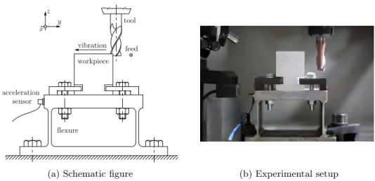
(a) Schematic figure (b) Experimental setup
Figure 2: Schematic figure and experimental setup for milling with single-degree-of- freedom experimental system.
2.1 Stability criterion
Based on the semi-discretization method presented in [6], the system stability is ap- proximated by means of the finite-dimensional transition matrix Φ. The detailed construction ofΦ can be found in the Appendix. The eigenvalues of Φ, which are called characteristic multipliers (or Floquet multipliers), are calculated from the char- acteristic equation det(µI−Φ) = 0. The system is stable if all the multipliersµiare located inside the unit circle of the complex plane, that is|µi|<1 for alli.
3 System identification
In this section, we present an improved validation method, which provides not only qualitative results (stable/unstable), but also a quantitative measure of stability. The key idea is to approximate the modulus of the largest Floquet multiplier based on the measurement data. In this case, the experimental results can be compared directly to the theoretical predictions obtained by the semi-discretization method.
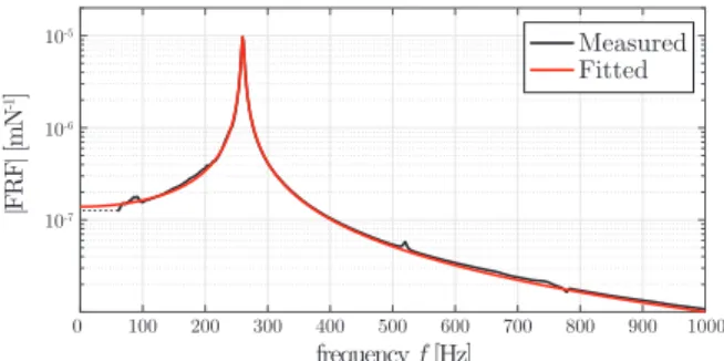
The experimental procedure is presented for a milling operation of a flexible struc- ture. The workpiece is clamped onto the top of a flexure, which was designed to mimic the dynamics of a single-degree-of-freedom system (SDoF). The sketch and the photo of the experimental setup are presented in Fig. 2a and 2b, respectively. The structure is flexible only alongydirection and can be considered to be rigid in the feed direction x, as it is presented in Fig. 1. The measured FRF and the fitted FRF can be seen in Fig. 3, which shows that the single-degree-of-freedom approximation is satisfactory for the demonstration (data corresponding to the fitted model can be found in Sec.
4).
To be able to analyse the perturbed vibration component η(t) in Eq. (9), it is necessary to excite the system during the milling operation [32]. The flexure is per- turbed with an impact (hammer blow) inydirection and the response is measured by means of a piezoelectric accelerometer. To analyse the displacement and the velocity
0 100 200 300 400 500 600 700 800 900 1000
frequency f [Hz]
10-7 10-6
10-5 Measured
Fitted
|FRF| [mN-1]
Figure 3: Measured and fitted frequency response functions
signals, double and single integration in frequency domain are used together with an appropriate high-pass filter.
3.1 Comb filter
According to the theory, the stability properties and the characteristic multiplier can be determined from the perturbed termη(t), which is superimposed to the periodic forced vibration yp(t), in Eq. (9). For this purpose, the measured signal has to be separated into two parts, too.
To obtain the perturbed term, the periodic vibration has to be subtracted from the measured signal. The separation is based on the so-called comb filter, which is a widely used method to eliminate the periodic components from a signal [35]. If a periodic vibration with periodτwas a purely harmonic function, then it would be presented as a single peak in the frequency domain, which is located at the tooth passing frequency ftp= 1/τ. Since the theoretical cutting force is not a continuous function due to the tool engagement, therefore the corresponding periodic forced vibration contains the tooth passing frequency and its integer multiples (higher harmonics, see Fig. 4.a). In order to separate or subtract the periodic vibration, the tooth passing frequency and its higher harmonics have to be filtered out from the original signal. It can easily be done by means of the comb filter, which is usually described in the following form
H(ω) = 1−βexpiπωn fb
, (12)
where β is a positive scaling factor, n is the filter order or the number of notches minus 1 andfb is the filtered base frequency (see Fig. 5.a). Note that in this study, the DSP System Toolbox of MATLAB and the infinite impulse response (IIR) comb filter were applied.
In this paper, the base frequencyfbis the tooth passing frequencyftp, which can be identified from the pre-set spindle speed Ω (see black square in Fig. 4) as
ftp= Ω
2πN. (13)
However, this frequency would not be accurate enough, since in practice, there is usually a small deviation (∼0.1%) between the pre-set and the realized spindle speeds.
Figure 4: Accurate detection of the spindle speed. Black square: pre-set spindle speed, red triangle: first dominant harmonic of the measured signal, green circle: adequate accurate spindle speed. Panel (b) and (c) represent small error in the detected spindle speed, which can be magnified significantly for the higher harmonics
Consequently, the precise identification of the realized tooth passing frequencyfbtp(or the realized spindle speedΩ) is required for appropriate filtering (see [19]). An initialb estimation for the realized spindle speed can be calculated from the first dominant harmonic of the measured signal in frequency domain (see red triangles in Fig. 4.ab).
Even if the frequency resolution is sufficiently accurate and the detected tooth passing frequency seems to be close to the exact one (see the green circle and red triangle in Fig. 4.b), the comb filter usually does not work properly, since even a small error can be magnified significantly at the higher harmonics (Fig. 4.c). It is therefore advisable to detect a peak at a selected mth higher harmonic of the tooth passing frequencymftp. In practice,m= 50 was found to be an appropriate choice, because the accuracy offtp is 1/m= 2% of the frequency resolution.
Important to note that if run-out occurs in the cutting process, which means that the cutting edges of a multi-edge milling tool cut different chip thickness during one revolution, then the first peak in the spectrum of the resulting vibration is not the tooth passing frequency (ftp =NΩ/(2π)), but the spindle frequency (fs = Ω/(2π)).
In these situations, the principal period of the system is 1/fsand the base frequency fbfor the comb filter is the spindle frequencyfs
fb= Ω
2π. (14)
The effect of the comb filter is visualized in Fig. 5. The blue curve is the spectrum of the original signal, and the red one is the filtered signal. It can be seen on the filtered
Figure 5: (a) Transfer function of the applied comb filter and (b) the filterred spectrum of the measured signal. Parameters for the filtering: base frequencyfb = 261.7379 Hz, Shelving Filter Order SFO=5, Bandwith BW=5 Hz, Bandwith Gain GBW=−4
signal, that the amplitude of the tooth passing frequency and its higher harmonics are eliminated and the remaining peaks corresponding to the perturbed term, only. The time function of the perturbed term can be obtained by means of applying inverse Fourier Transformation of the filtered spectrum (see, for instance, Fig. 6.c).
Note that the periodic term can be obtained in two different ways. One of them is to subtract the perturbed term from the original signal, as follows
yp(t) =y(t)−η(t). (15)
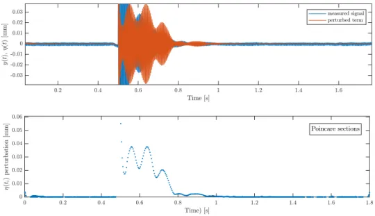
The other one is to apply directly the so-called notch filter, which is the counterpart of the comb filter, therefore it eliminates every frequency component except the base frequency and its higher harmonics. To summarize briefly, the measured signal of the system is separated into periodic and perturbed terms according to Eq. (9), as it is shown in Fig. 6. On the top figures, the original measured signaly(t) is visualized, where there is a hammer blow after 1 second on the left panel. On the middle figures, blue curve represents the original signaly(t) and grey plot shows the periodic vibration yp(t) obtained by the notch filter. The bottom figures represent only the perturbed termη(t), obtained by the comb filter.
3.2 Determination of the dominant multiplier
In this subsection, the exponential decay of the perturbed term is analysed. Accord- ing to the theory of linear time-periodic delay-differential equations, the system has infinitely many characteristic multipliers (µi), each defines a decay ratio. This decay ratio is proportional to the logarithm of the multipliers (µi), which is proved [36] to tend to zero asitends to infinity, similar to the decay ratios of the vibration modes of continuous beams.
In case of an impulse excitation (hammer blow) all the modes are excited in the time delayed system, similarly to a continuous beam. Although the system has infinite number of characteristic multipliers, at the stability boundary usually there is only
0.75 1.25 1.5 1.75
0.75 1.25 1.5 1.75
0.75 1.25 1.5 1.75
Figure 6: Measurement representation for stable (left panel) and unstable (right panel) cases. On plot (a): blue is the measured displacement signal. On plot (b):
gray is the forced periodic vibration component of the signal obtained by means of notch filter. On plot (c): red is the perturbed motion of the measurement obtained by means of comb filter. Parameters for the stable case (left panel): n= 8100 rpm, ap= 0.75 mm, ae = 1 mm, fz = 0.05 mm; Parameters for the unstable case (right panel): n= 8425 rpm, ap= 1 mm,ae= 1 mm, fz= 0.05 mm
one critical real multiplier (or a critical complex conjugate pair of multipliers) on the unit circle at a time in a generic case, which refers to a single undamped mode.
Based on the above statements, it can be assumed, that the transient vibrations of the non-critical modes decay relatively fast. Therefore the envelopes of the transient vibrations are well-approximated by an exponential function corresponding to the dominant mode only.
3.3 Poincare section
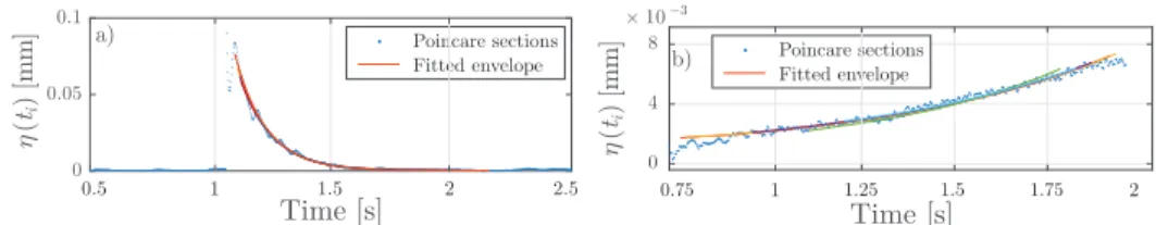
The exponential envelope characterized by the decay ratio of the dominant mode can be attained by tracking the local maximum of the perturbed displacement signal, which can be found at time instants where the perturbed velocity is zero (see blue dots in Fig. 7, which are the counterparts of panel c) in Fig. 6). This method realises a Poincare section, which is a standard tool in the analysis of nonlinear dynamical sys- tems [37]. Note that this leads to a well-conditioned point set, because the perturbed displacement and velocity are calculated from the original measured acceleration by means of numerical integration in frequency domain.
The determination of the dominant multiplier is based on an exponential curve- fitting technique. To solve the least-squares optimal curve-fitting problem, it can be given for the sampled data in a discrete form as
minγ
X
i
(F(γ, ti)i−η(ti))2, (16) where the subscript i stands for the discrete representation form according to the Poincare data set,η(t) is the perturbed term, γ is the fitted parameter and F(γ) is
Time [s]
()ti ()ti
Time [s]
Figure 7: Envelope of the perturbed term and fitted exponential curves
the trial exponential function given as
F(γ, ti) =η0eγti, (17)
whereη0is the initial amplitude of the perturbed term for the curve-fitting technique.
After a successful fitting of η0 and γ (see fitted exponential curves in Fig. 7), the modulus of the dominant multiplier is the largest, and it can be calculated as
max|µ|= abs(eγτ). (18)
Close to the stability boundary (in other words, near to the case in which the critical multiplier almost crosses the unit circle), the amplitude of the solution segment decreases very slowly. If the critical multiplier just passes the stability boundary, then the amplitude of the response is increasing very slowly till the cutting edges leave the material. This is the so-called fly-over effect, which saturates the vibration amplitude and ends up in an often chaotic (chatter) vibration [38] (see the right panel of Fig.
9). In this case, there is no need to excite the system by hammer blow to trace the perturbed term. The slowly increasing amplitude gives an opportunity to fit an exponential curve to its envelope, (see Fig. 7.b). This phenomenon is visualized in the right panel of Fig. 6c, where a slight increase in the amplitude of vibration can be observed (0.75-2.2 s).
After this, a hammer blow is initiated at around 2.2 s (see Fig. 8), and an expo- nentially decreasing vibration amplitude can be recognized. In fact, it is also visible in Fig. 8 (after the periodic vibration is subtracted by means of comb filter) that the amplitude is increasing before the hammer blow, which refers to the presence of an unstable mode with |µ|>1. Thus, there is no need to impact to determine the magnitude of the (unstable) Floquet multiplier.
After the hammer blow, however, an exponentially decreasing vibration amplitude can be bserved. This decreasing characteristic does not mean that the small amplitude periodic forced vibration of the machining process is stable; it is still linearly unstable.
The decreasing amplitude does not converge to the periodic forced vibration, but it converges to a chatter vibration [38, 39], which corresponds to a stable chaotic attractor (see Fig. 9). By looking only at the initial converging behaviour of the vibration signal after the impact, there is a risk that a slightly unstable condition is classified as stable, which would be incorrect. In order to avoid this problem, first, the signal range before the impact should be analysed, and if this section already shows unstable behaviour, then the signal after the hammer hit must be omitted.
In some special cases, if we cannot realise the slightly unstable motion before the hammer hit, we can still recognise the attracting chatter vibration if the filtered
Converges to chatter vibration Linearly unstable
machining process
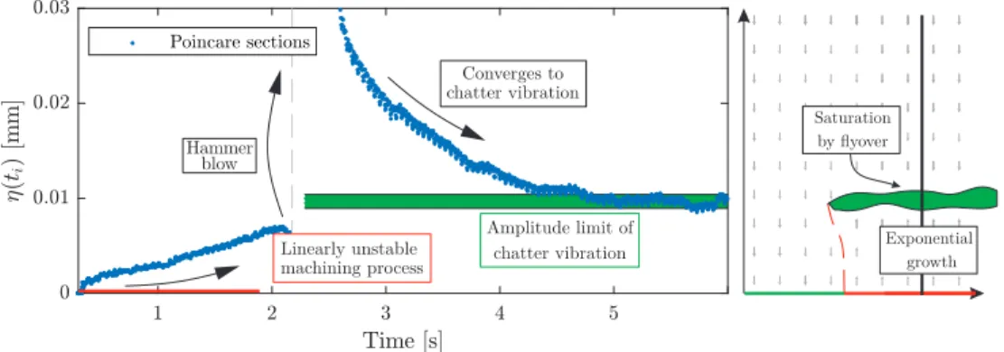
Figure 8: Unstable measurement case where the periodic vibration is subtracted by means of comb filter. At the beginning: increasing amplitude of the linearly unstable machining process; after hammer blow: stable chaotic attractor (chatter).
Parameters: n= 8425 rpm, ap= 1 mm,ae = 1 mm,fz= 0.05 mm
Amplitude limit of
chatter vibration Exponential
growth Saturation by flyover
Figure 9: Envelope of the unstable measurement case (left panel), and schematic figure of the solution (right panel). Parameters: n= 8425 rpm,ap= 1 mm, ae = 1 mm,fz= 0.05 mm
signal amplitude does not converge to 0. In this special case, we cannot estimate Floquet multiplier neither before the hammer hit nor after it, but we still can identify the chatter vibration. With the above described procedure, an unmanned expert monitoring system can still be established.
If a parameter point selected far from the stability boundary in the unstable domain, then the increasing vibration reaches the chaotic attractor (chatter motion) within a very short time, which is insufficient to extract the dominant characteristic multiplier. However, it is usually not necessary to determine the exact quantitative value of the multiplier, because this range is far away from the area of interest (the stability boundary).
4 Case study
The above described measurement technique is applied in a case study, where the dominant characteristic multiplier is determined for a set of different spindle speeds.
During one peripheral milling test along straight path, multiple excitations (hammer blows) were performed. The curve-fitting method is applied with several different time ranges of the perturbed term to eliminate the influence of the subjective human time selection. In this way, the deviation of the fitted values are also determined.
The measured multipliers are compared to the theoretically calculated ones, de- scribed in Sec. 2. For the cutting tests, Aluminum 2024-T351 material was selected.
In order to fit cutting parameters, cutting tests were performed with radial immersion ae= 2 mm, feed per tooth fz = 0.02, 0.04 and 0.06 mm/tooth and axial immersion ap = 1 and 2 mm. The TIVOLY P615H endmill had diameter D = 16 mm, num- ber of flutes N = 2, helix angle β = 30◦ and rake angle κ = 90◦. Since, it nearly matches the cutting conditions of the experiments, the resulted cutting parameters are expected to provide reasonably good approximation for the cutting force. Note that due to the softening nonlinear cutting force characteristics against chip thick- ness (see [40]), the fitted linear cutting coefficients are somewhat larger than their expected standard values for the relatively low radial immersion and feed per tooth rate. During the measurement, the workpiece was mounted on a Kistler dynamometer plate [41]. The resultant tangential and radial force coefficients areKt= 2.203·109 N/m2 and Kr = 1.723·109 N/m2, respectively. The frequency response function of the flexure is measured by means of impact tests. The fitted modal parameters of the single-degree-of-freedom system arem= 2.701 kg,ζ= 0.71 % andωn= 259.96 Hz.
During the experiment, the tool was attached to a spindle adapter BT30 ER16 on a three axis NCT EMR-610MS machine tool. The experiments were carried out at radial immersion ae = 1 mm, axial immersion ap = 2 mm, with a down-milling operation in the spindle speed range [7900, 8100] rpm. The response of the SDoF flexure was acquired by NI cDAQ-9178 Chassis with NI 9234 Module at 52kHz sampling rate and PCB 352C23 type acceleration sensor. The multipliers were calculated at least 5 times for each spindle speed with different time segments, as it is shown with different curves in Fig. 7. It was necessary, because all measurement data are loaded with uncertainty and inaccuracy coming from the data acquisition system and the fitted cutting force coefficients. Furthermore, the selected ranges for the curve fitting in Sec. 3.3 have some influence on the fitted modulus of the characteristic multipliers.
The actual value of the detected multipliers are approximated by the average for every spindle speeds and they are presented together with their 95% confidence level in Table 1. The results are also shown in Fig. 10. The theoretically predicted variation of the dominant multiplier (based on the semi-discretization method and the fitted FRF function in Fig. 3) is visualized with thick red curve, and the measured multipliers are plotted with black dots together with the error bars at 95% confidence level. Note that these deviations are negligible compared to the variation along the curve. However, close to the stability boundary, the deviations are much larger and the data points are off of the visible tendency. These data points (denoted by gray dots in right panel of Fig. 10) should have been neglected due to the insufficient fitting as described in the end of Sec. 3.3.
In order to explain the source of this error, the schematic bifurcation diagram in
Fitted curve with 95% confidence
interval
n n
Figure 10: Results of the measured multipliers compared to the theoretical ones.
Chatter vibration
large hit is ok no hit
Linear stability boundary
Unstable stat. motion unsafe zone
Stable stationery motion
vibration amplitude
Figure 11: Schematic figure of the bistable zone. Gray arrowfield shows the attraction zone. Green and red horizontal lines represents the stable and unstable stationary motion, respectively. Red dashed line is an unstable periodic motion which separates two stable solution (stationary motion and chatter vibration).
Fig. 11 represents the behaviour of the vibration near the linear stability boundary.
The horizontal parameter axis can be divided into 3 parts. At the left and right side, where the periodic motion is linearly stable or linearly unstable, respectively, the Floquet multipliers can be identified by means of the proposed method. The param- eter domain in between is called unsafe or bistable zone since two attractive motions coexist: stable cutting and (mathematically stable) chatter, which are separated by an unstable periodic motion [39, 38]. In this range, the vibration can jump from the linear attraction zone to the chatter motion due to a large-enough perturbation.
Unfortunately, in practise, a really small impact can cause this type of switch and the linear attraction zone cannot be analysed through the curve fitting method here.
Therefore the source of the error near the stability boundary could be the existence of the unmodelled unsafe (bistable) zone. Neglecting these unsuitable data points, there are good correlations between the measured data and the theoretically predicted multipliers.
Moreover, if a curve fits to the data, the stability boundary can be predicted with
Figure 12: Top panel: measurement representation for period doubling vibration with significant run-out effect. Blue is the measured displacement signal and red is the perturbed motion of the measurement obtained by means of comb filter. Bottom panel: envelope of the perturbed term from the Poincare sections.
very high accuracy. In this case study, a second order polynomial was fitted to the measured data points in the formf(n) =a0+a1n+a2n2. The stability boundary ˜n can be given byf(˜n) = 1. The fitted coefficientsaiand the coefficient of determination R2 are presented in Table 2. The measured stability boundary is ˜n= 7995 rpm with deviance n2σ = 14 rpm, which is less then 0.2%, while the theoretically predicted value isn= 8000 rpm.
Note that the theoretically predicted multipliers are in the confidence interval on the stable side, however, at the unstable part, the calculated data underestimate the theoretical ones. One explanation for this can be, that the stable chaotic attractor and its attraction zone effect the growth ratio near to the unstable periodic orbit [38].
An important advantage of the proposed method is that it is not required to reach spindle speed ranges corresponding to chatter vibration to detect the stability boundary. If there are measured points and detected multipliers sufficiently close to the stability boundary still in the stable domain, then the stability boundary can be predicted by means of extrapolation.
However, the proposed method has some disadvantages: at the peaks of the sta- bility boundaries (where two lobes intersect each other), 2 different multipliers cross the unit circle, therefore, it is not sufficient to approximate the transient vibration with 1 critical mode only.
In some cases of Hopf bifurcation close to the asymptote of the stability lobe (see the Hopf lobe in Fig. 10), the time period of the arising self-excited vibration is close to the tooth passing period, that is, the chatter frequency is approximately equal to the
Realized spindle speed Characteristic multiplier Mean value 95% confidence interval
bn |µ| 2σ
(rpm) (1) (1)
7902.39 0.9820 3.120×10⁻³
7927.13 0.9887 2.616×10⁻³
7952.20 0.9917 2.756×10⁻³
7962.34 0.9961 0.310×10⁻³
7972.14 0.9986 0.834×10⁻³
7977.05 0.9970 2.086×10⁻³
7982.35 0.9981 0.798×10⁻³
8012.01 1.0025 1.526×10⁻³
8022.02 1.0015 2.260×10⁻³
8027.28 1.0037 1.450×10⁻³
8032.19 1.0029 0.980×10⁻³
8052.34 1.0055 2.924×10⁻³
8077.02 1.0073 2.488×10⁻³
7992.18 1.0132 8.018×10⁻³
8002.04 1.0080 8.862×10⁻³
8001.94 1.0063 6.176×10⁻³
Table 1: Mean value and standard deviation (at the level of confidence of 95%) of the measured data. Note that the last 3 measurement points are dropped out.
tooth passing frequency:fch−ftp < BW. Since the applied comb filter eliminates the tooth passing frequency, and all of its higher harmonics and neighbouring frequency components within bandwith BW, the useful information is filtered out from the original measurement signal, too.
Additional cons of the proposed method can be evolved for stability boundary identification at flip (period-doubling) bifurcation (see the flip lobe in Fig. 10) in case when the run-out effect is significant and endmill with even number of flutes is used.
Flip bifurcation results that the time period of the arising self excited vibration is double of the tooth passing period, that is, the chatter frequency is approximately equal tofch =ftp(j+ 1/2), j ∈ N0. Due to the presence of the run-out effect, the base frequency of the comb filter is the spindle frequency (see Eq. 14), therefore, its higher harmonics match with the chatter frequency, and the relevant information for the fitting of the Floquet multipliers is fallen out through the filtering. A flip- type measurement case is presented in Fig. 12, where the run-out effect cannot be neglected during the measurement. In this situation, the periodic term can sufficiently be subtracted with the comb filter, but the perturbed part is inadequate for the curve fitting algorithm, therefore the multiplier identification is unsuccessful. Further research is needed to resolve this problem.
a2 a1 a0 R2 n˜
(rpm−2) (rpm−1) (1) (1) (rpm)
−6.15247×10⁻⁷ 9.96882×10⁻³ −39.3741±1.8578×10⁻³ 0.9653 7995±14 Table 2: Coefficients of the fitted curve with 95% confidence level. Coefficient of determinationR2 and the stability boundary.
5 Conclusion
In this paper, a new method is introduced to identify the stability boundaries of cutting operations directly from vibration measurements. The standard methods known from the literature determine the stability properties for a given combination of manufacturing parameters with great uncertainty that is usually unacceptable in industry. In this paper, an improved prediction was proposed to estimate the stability lobe diagram by means of the modulus of the dominant Floquet multiplier. The method is based on the investigation of the transient vibrations, which are generated by operational impact tests. The response of the system is captured by acceleration signals, from which the perturbation about the periodic orbit can be separated by the use of a comb filter.
With this quantitative measure of the machining process, the variation of the sta- bility limit can also be traced without switching between stable and unstable cutting operations. The stability boundary can be determined precisely by means of interpo- lation between measurement points, furthermore, extrapolation can also be used to predict the distance from the stability boundary based on stable measurement points only.
The efficiency and accuracy of the proposed methodology were validated by means of peripheral milling tests. These results support the technology design to identify those parameters where the milling process is stable.
Note that all these steps can be obtained from other signals, but the signal/noise ratio are out of the scope of this work, which can be a significant question for different type of measurements (e.g.: microphone, acceleration measurement on the spindle house).
It is still left for future research to improve the method in order to be capable to detect the dominant Floquet multiplier at certain stability lobe boundaries, where the arising chatter frequency and the tooth passing frequency are almost equal. This problem can also appear typically when the stability boundary is related to a period doubling vibration and even fluted tool is applied with run-out. An automatized impact excitation is also to be developed to improve industrial applicability.
6 Acknowledgements
This paper was supported by the Hungarian Scientific Research Fund - OTKA PD- 112983 and the Janos Bolyai Research Scholarship of the Hungarian Academy of Sciences. The research leading to these results has received funding from the Euro- pean Research Council under the European Unions Seventh Framework Programme
(FP/2007-2013) / ERC Advanced Grant Agreement n. 340889. Supported by the UNKP-17-3-I. New National Excellence Program of the Ministry of Human Capaci-´ ties.
References
[1] S. Tobias,Machine-tool Vibration. 1965.
[2] J. Tlusty and L. Spacek, Self-excited vibrations on machine tools. Prague. in Czech.: Nakl. CSAV, 1954.
[3] Y. Altintas and E. Budak, “Analytical prediction of stability lobes in milling,”
CIRP Ann-Manuf Techn, vol. 44, pp. 357–362, 1995.
[4] E. Budak and Y. Altintas, “Analytical prediction of chatter stability in milling, part i: General formulation,” J Dyn System ASME, vol. 120, pp. 22–30, 1998.
[5] D. Bachrathy and G. Stepan, “Improved prediction of stability lobes with ex- tended multi frequency solution,”CIRP Ann-Manuf Techn, vol. 62, pp. 411–414, 2013.
[6] T. Insperger and G. Stepan,Semi-discretization for time-delay systems, vol. 178.
New York: Springer, 2011.
[7] Y. Ding, L. M. Zhu, X. J. Zhang, and H. Ding, “A full-discretization method for prediction of milling stability,”Int J Mach Tool Manu, vol. 50, pp. 502–509, 2010.
[8] X. J. Zhang, C. H. Xiong, Y. Ding, M. J. Feng, and Y. L. Xiong, “Milling stability analysis with simultaneously considering the structural mode coupling effect and regenarative effect,”Int J Mach Tool Manu, vol. 53, pp. 127–140, 2012.
[9] M. Zatarain and Z. Dombovari, “Stability analysis of milling with irregular pitch tools by the implicit subspace iteration method,” Int J Dynam Control, vol. 2, pp. 26–34, 2014.
[10] E. A. Butcher, O. A. Bobrenkov, E. Bueler, and P. Nindujarla, “Analysis of milling stability by the chebyshev collocation method: algorithm and optimal stable immersion levels,” J Comput Nonlinear Dynam, vol. 4, no. 031003, 2009.
[11] G. Totis, P. Albertelli, M. Sortino, and M. Monno, “Efficient evaluation of pro- cess stability in milling with spindle speed variation by using the chebyshev collocation method,” J Sound Vib, vol. 333, pp. 646–668, 2014.
[12] F. A. Khasawneh and B. P. Mann, “A spectral element approach for the stability of delay systems,”Int J Numer Meth Eng, vol. 87, pp. 566–952, 2011.
[13] P. V. Bayly, J. E. Halley, B. P. Mann, and M. A. Davies, “Stability of interrupted cutting by temporal finite element analysis,” Journal of Manufacturing Science and Engineering, vol. 125, pp. 220–225, 2003.
[14] N. D. Sims, B. Mann, and S. Huyanan, “Analytical prediction of chatter sta- bility for variable pitch and variable helix milling tools,” Journal of Sound and Vibration, vol. 317, no. 3, pp. 664 – 686, 2008.
[15] D. Hajdu, T. Insperger, and G. Stepan, “Robust stability analysis of machining operations,” The International Journal of Advanced Manufacturing Technology, vol. 88, no. 1, pp. 45–54, 2017.
[16] Y. Altintas, Manufacturing Automation - Metal Cutting Mechanics, Machine Tool Vibrations and CNC Design, Second Edition. Cambridge: Cambridge Uni- versity Press, 2012.
[17] R. Du, M. A. Elbestawi, and B. Ullagaddi, “Chatter detection in milling based on the probability distribution of cutting force signal,” Mechanical Systems and Signal Processing, vol. 6, pp. 345–362, 1992.
[18] Y. Fu, Y. Zhang, H. Zhou, D. Li, H. Liu, H. Qiao, and X. Wang, “Timely online chatter detection in end milling process,”Mechanical Systems and Signal Processing, vol. 75, pp. 668–688, 2016.
[19] E. Kuljanic, M. Sortino, and G. Totis, “Multisensor approaches for chatter de- tection in milling,”Journal of Sound and Vibration, vol. 312, pp. 672–693, 2008.
[20] M. Shiraishi, “Scope of in-process measurement, monitoring and control tech- niques in machining processes - part 3: In-process techniques for cutting pro- cesses and machine tools,”Precision Engineering, vol. 11, pp. 39–47, 1989.
[21] T. Delio, J. Tlusty, and S. Smith, “Use of audio signals for chatter detection and control,”Journal of Engineering for Industry, vol. 114, no. 2, pp. 146–157, 1992.
[22] T. L. Schmitz, “Chatter recognition by a statistical evaluation of the syn- chronously sampled audio signal,” Journal of Sound and Vibration, vol. 262, pp. 721–730, 2003.
[23] O. O. Khalifa, A. Densibali, and W. Faris, “Image processing for chatter identi- fication in machining processes,”Int J Adv Manuf Technol, vol. 31, pp. 443–449, 2006.
[24] Y. Altintas and P. K. Chan, “In-process detection and suppression of chatter in milling,” International Journal of Machine Tools and Manufacture, vol. 32, no. 3, pp. 329–347, 1992.
[25] E. Kuljanic, G. Totis, and M. Sortino, “Development of an intelligent multisensor chatterdetection system in milling,” Mechanical Systems and Signal Processing, vol. 23, pp. 1704–1718, 2009.
[26] Y. Liao and Y. Young, “A new on-line spindle speed regulation strategy for chat- ter control,” International Journal of Machine Tools and Manufacture, vol. 35, no. 5, pp. 651–660, 1996.
[27] B. P. Mann and K. A. Young, “An empirical approach for delayed oscillator sta- bility and parametric identification,”Proceedings of the Royal Society A, vol. 462, pp. 2145–2160, 2006.
[28] A. Honeycutt and T. L. Schmitz, “A new metric for automated stability identi- fication in time domain milling simulation,” Journal of Manufacturing Science and Engineering, vol. 138, no. 074501, 2016.
[29] J. Munoa, X. Beudaert, Z. Dombovari, Y. Altintas, E. Budak, C. Brecher, and G. Stepan, “Chatter suppression techniques in metal cutting,” vol. 65, pp. 785–
808, 66th General Assembly of the International-Academy-for-Production- Engineering, Guimaraes (Portugal), 21 Aug 2016 - 27 Aug 2016, CIRP, 2016.
[30] G. Quintana and J. Ciurana, “Chatter in machining processes: A review,” In- ternational Journal of Machine Tools and Manufacture, vol. 51, pp. 363–376, 2011.
[31] D. A. W. Barton, “Control-based continuation: Bifurcation and stability analysis for physical experiments,” Mechanical Systems and Signal Processing, vol. 84, pp. 54–64, 2017.
[32] K. D. Murphy, P. V. Bayly, L. N. Virgin, and J. A. Gottwald, “Measuring the stability of periodic attractors using perturbation-induced transients: Applica- tions to two non-linear oscillators,” Journal of Sound and Vibration, vol. 172, pp. 85–102, 1994.
[33] A. K. Kiss, D. Bachrathy, and G. Stepan, “Experimental determination of dom- inant multipliers in milling process by means of homogeneous coordinate trans- formation,” (Cleveland, Ohio, USA), pp. 1–8, American Society of Mechanical Engineers, 29th Conference on Mechanical Vibration and Noise, In Press, 2017.
[34] Z. Dombovari and G. Stepan, “The effect of helix angle variation on milling stability,” Journal of Manufacturing Science and Engineering, vol. 134, no. 5, p. 051015, 2012.
[35] L. Jackson, Digital Filtering and Signal Processing. Boston: Kluwer Academic Publishers, 1986.
[36] Q. Xu, G. Stepan, and Z. Wang, “Numerical stability test of linear time-delay sys- tems of neutral type, in press,” inAdvances in Delays and Dynamics; Time De- lay Systems Theory, Numerics, Applications, and Experiments, vol. 7, Springer, 2016.
[37] J. Guckenheimer and P. Holmes, Nonlinear Oscillations, Dynamical Systems, and Bifurcations of Vector Fields. New York: Springer, 1983.
[38] Z. Dombovari and G. Stepan, “On the bistable zone of milling processes,”Philo- sophical Transactions of the Royal Society of London A: Mathematical, Physical and Engineering Sciences, vol. 373, no. 2051, 2015.
[39] H. M. Shi and S. A. Tobias, “Theory of finite amplitude machine tool instability,”
International Journal of Machine Tool Design and Research, vol. 24, no. 1, pp. 45 – 69, 1984.
[40] G. Stepan, Z. Dombovari, and J. Munoa, “Identification of cutting force char- acteristics based on chatter experiments,” CIRP Ann-Manuf Techn, vol. 60, pp. 113–116, 2011.
[41] O. Kienzle, “Spezifische schnittkrfte bei der metallbearbeitung,”Werkstattstech- nik und Maschinenbau, vol. 47, pp. 224–225, 1957.
Appendix: Semi-discretization
The state-space form of the governing equation (10) with the state vector v(t) = (η(t) ˙η(t))> reads
v(t) =˙ A(t)v(t) +B(t)u(t),
u(t) =Dv(t−τ), (19)
where
A(t) =
0 1
−(ωn2+G(t)m ) −2ζωn
, B(t) = 0
G(t) m
, D= 1 0
. (20) Note that the principal period of the coefficient matricesA(t), B(t) is the sameτ as the time delay. Based on the semi-discretization method presented in [6], the periodic coefficients are approximated by piece-wise constant terms, i.e.
Ak= 1 h
Z tk+1
tk
A(t)dt, Bk = 1 h
Z tk+1
tk
B(t)dt, (21) wherek= 1,2. . . p,tk=kh,τ=ph,his the discretization step andpis the number of the discretization steps over the principal periodτ. Based on the discretized solution of (19), assuming piecewise constant coefficient matrices, the linear mapping which projects the solution to the next time step can be formulated as
zk+1=Gkzk, (22) wherezk = (v(tk)>u(tk−1) · · · u(tk−p))> and the construction of Gk is detailed in [6]:
Gk =
Pk 0 · · · 0 Qk
D 0 · · · 0 0 0 I · · · 0 0 ... ... . .. ... ...
0 0 · · · I 0
, Pk = eAkh, Qk= Z h
0
eAk(h−s)Bkds, (23)
where I denotes the 1-dimensional identity matrix. Finally, the system stability is approximated by means of the finite-dimensional transition matrixΦas
zk+p=Φzk=Gk+p−1Gk+p−2· · ·Gkzk. (24)