Accepted for publication inApplied Mathematical Modelling (13. Dec. 2017)
The publication is available at Elsevier viahttps://doi.org/10.1016/j.apm.2017.12.029
Numerical methods for the stability of time-periodic hybrid time-delay systems with applications
David Lehotzky
∗,a, Tamas Insperger
a, and Gabor Stepan
baDepartment of Applied Mechanics, Budapest University of Technology and Economics and MTA-BME Lend¨ulet Human Balancing Research Group, 1111 Budapest, Hungary
bDepartment of Applied Mechanics, Budapest University of Technology and Economics, Hungary, 1111, Budapest, Muegyetem rkp. 3.
Abstract
This paper extends two numerical methods for the stability analysis of a class of time-periodic hybrid time-delay systems. In particular, the pseudospectral tau and spec- tral element methods are extended to hybrid systems. The analyzed delay-differential equation involves delayed terms with both continuous and piecewise constant arguments, in other words, it involves delays both without and with zero-order hold, respectively.
The analyzed class of hybrid systems can be used to describe time-periodic hereditary processes subjected to digital feedback control. The proposed numerical algorithms are applied to the mathematical models of haptic systems and milling processes subjected to digital feedback control.
Keywords: time-delay system; hybrid system; time-periodic system; digital control; haptic system;
milling process
∗Corresponding author
E-mail address: lehotzky@mm.bme.hu
1 Introduction
As the importance of delay effects has been realized in several engineering and biological appli- cations, the attention to the analysis of time-delay systems has increased in the recent decades.
Time delay is inherently present in machine tool vibrations [1], control systems [2], traffic dy- namics [3], human balancing [4], population dynamics [5] or epidemiology [6], just to mention a few examples. The local stability analysis of these time-delay systems provides the primary characteristics of their behavior around stationary states. Consequently, several analytical and numerical methods have been developed for local stability analysis. For instance, the D- subdivision method [7] gives a closed form solution for the stability boundaries of autonomous delay-differential equations in the space of system parameters. While closed form solutions can be derived for the stability boundaries of most autonomous systems, the stability analysis of time-periodic systems usually requires numerical approximation techniques, especially in the presence of time-delays. The related literature provides many numerical methods for the sta- bility analysis of time-periodic time-delay systems, such as the semi-discretization method [8], full discretization method [9], spectral element method [10] or the pseudospectral collocation method [11, 12], just to mention a few examples.
In digitally controlled mechanical systems (see e.g. [13]), the state variables in the governing equations appear with piecewise constant arguments due to sampled data hold in the feedback loop, which results in a hybrid system. Here, the terms with piecewise constant arguments will be referred as terms with discrete delays. The open-loop system can also incorporate delayed terms, whose arguments are continuous functions of time. In the following, these terms will be referred as terms with continuous delays.
Mathematical models involving both discrete and continuous delays can arise in case of coupled haptic systems (see e.g. [14, 15]), where the haptic device is subjected to both human interaction and digital feedback control. In these models, continuous delay terms are present due to the reaction delay of the human operator, while discrete delay terms are originated from the sampling and actuation scheme of the digital controller. Further examples for hybrid time- delay systems can be taken from the field of machine tool vibrations. Here the continuous delay is present due to the so-called regenerative effect of the cutting process [16], while the discrete delays are originated from the feedback control of the workpiece-tool system and from the feedback loop of the active damper used for the vibration suppression of the cutting tool.
In spite of the relevant applications of time-delay systems subjected to digital feedback control, their numerical stability analysis is not well-established in the engineering literature. In this paper, two existing numerical methods, the pseudospectral tau (PT) method and the spectral element (SE) method are extended for the stability analysis of linear hybrid time-periodic time-delay systems.
The extended numerical methods are tested on two engineering applications. First, the math- ematical model of a coupled haptic system is analyzed. To our knowledge, stability analysis of coupled haptic systems has been carried out in the literature either with the omission of discrete delay terms or with the substitution of continuous delay terms by continuous non- delayed terms. Therefore, this paper presents the stability analysis of a coupled haptic system considering continuous and discrete delays simultaneously.
The second application is for milling processes subjected to active damping. In the machining literature, such processes have been modeled using continuous, non-delayed feedback terms in the control input. However in practice, active damping is realized using a digital feedback controller which necessitates the incorporation of discrete delay terms in the governing equa- tions. In this paper, the stability analysis of milling processes subjected to active damping is performed with the consideration of discrete delay in the feedback loop.
2 The equation under analysis
In this paper the stability of the dynamical system
˙
x(t) =A(t)x(t) +
m
X
a=1
Ba(t)x(t−τa) +
n
X
b=0
Cbx(tj−b∆t), t∈[tj, tj+1), (1) is analyzed with initial condition
x(θ) = x0(θ), θ ∈[−τ,0], (2) where j ∈ N; x : [−τ,∞) → Rs; A, Ba : R → Rs×s; Cb ∈ Rs×s and A(t) = A(t+T), Ba(t) = Ba(t +T) ∀t, with T being the time-period of the periodic coefficients. The non- zero continuous delays are denoted by τa > 0, a = 1,2, . . . , m and the length of time history is τ = max(τ1, τ2, . . . , τm, n∆t). Equation (1) models the digital feedback control of a time- periodic system with system delays. The digital control applies state feedback via gain matrices Cb. The state is measured at each sampling instant tj +b∆t, j ∈N, b = 0,1, . . . , n; while the control input is updated at time instants tj = j∆T, j ∈ N, where ∆t is the sampling period and ∆T = v∆t is the actuation period, with v ∈ Z+ being the number of samples between two control input updates while Z+ denotes the set of positive integer numbers. The control input is held constant between the two endpoints of each actuation period in accordance with a zero-order hold. In this paper it is assumed that the calculation of the control input requires the knowledge of the state in n+ 1 consecutive sampling instants from domain [tj −n∆t, tj], therefore the state-feedback terms in (1) are subjected to delays. The employment of past samples aims to cover a broader group of control methods of delayed systems (involving e.g.
the finite spectrum assignment [17], Smith predictor [18], act-and-wait [19] and optimal control [20] methods), where not only the most recent samples but past samples or a weighted sum of past samples also contribute to the control law. In (1), x(t−τa), a = 1,2, . . . , m; are terms with continuous delays, while x(tj−b∆t),j ∈N, b= 0,1, . . . , n; are terms with discrete delays.
In case of a general choice for T and ∆T this system is quasi-periodic. In this paper it is assumed that T /∆T = σ/ρ, with σ, ρ ∈ Z+, thus Tp = σ∆T = ρT is the principal period of the system. Note that although (1) contains only constant continuous delays (pointwise delays), DDEs involving distributed continuous delay terms can also be approximated by (1) using numerical quadratures as introduced in [21].
The stability of (1) is determined by the characteristic multipliers of the monodromy operator U, which is defined as
xjTp =Ux(j−1)Tp, j =Z+, (3)
where function segmentxt is given by the shift
xt(θ) =x(t+θ), θ ∈[−τ,0]. (4)
Equation (1) is asymptotically stable if and only if all the characteristic multipliers of U are within the unit circle of the complex plane [22]. In the next section, the extension of the PT and the SE methods are presented for the matrix approximations of U.
3 Numerical stability analysis
This section details the application of the PT [23] and SE [21] methods for the approximation of the monodromy operator of the hybrid system (1). While the PT method discretizes the operator differential equation form, the SE method is based on the operator equation form of (1). For the approximation of the operator differential equation and the operator equation, both numerical techniques use the method of weighted residuals and the tau method. In this section, the main steps of the approximation schemes are given for the hybrid system (1). The full description of the PT and SE methods for continuous-time (non-hybrid) systems can be found in [23] and [21], respectively.
3.1 Pseudospectral tau method
Using function segment xt, (1) can be converted to the operator differential equation form x˙t=G(t)xt+Hxtj, t ∈[tj, tj+1), (5) where operatorsG(t) and Hare defined as
(G(t)ψ)(θ) =
(A(t)ψ(0) +Pm
a=1Ba(t)ψ(−τa) θ = 0,
d
dθψ(θ) θ ∈[−τ,0),
(Hψ)(θ) = (Pn
b=0Cbψ(−b∆t) θ = 0, 0 θ ∈[−τ,0),
(6)
with ψ : [−τ,0] → Rs. The PT method approximates function segment xt with its Lagrange interpolant ˜xt as
x˜t(θ) =
N+1
X
k=1
φk(θ)˜xt(θk), (7)
whereφk(θ) are the Lagrange base polynomials (see Appendix A) with{θk}N+1k=1 being the point set of interpolation. After the substitution of (7) to (1), the equation is multiplied with test functions {ψi(θ)}Ni=1 and integrated over domain θ ∈[−τ,0] according to the standard steps of the weighted residual method. In case of independent test functions, this gives N independent equations and the (N + 1)-st equation is obtained from the pointwise satisfaction of (5) at θ = 0. Consequently, the final form of the approximate system is given by
Ny(t) =˙ M(t)y(t) +Hy(tj), t ∈[tj, tj+1), (8) where, after coordinate transformation ζ = 2θ/τ + 1, the sub-matrices of N, M(t), H ∈ Rs(N+1)×s(N+1) and the sub-vectors of y(t)∈Rs(N+1)×1 are given as
Ni,k =
(IPN+1
q=1 φk(ηq)ψi(ηq)wq i= 1,2, . . . , N; Iφk(1) i=N + 1;
Mi,k(t) =
(I2τ PN+1 q=1
PN+1
l=1 φ0k(ζl)φl(ηq)ψi(ηq)wq i= 1,2, . . . , N; A(t)φk(1) +Pm
a=1Ba(t)φk(1−2τa/τ) i=N+ 1;
Hi,k =
(0 i= 1,2, . . . , N;
Pn
b=0Cbφk(1−2b∆t/τ) i=N + 1;
yk(t) = ˜xt(τ(ζk−1)/2),
(9)
where{ηq}N+1q=1 is the quadrature point set andwqare the weights used for numerical integration.
During computations, the point set of interpolation {ζk}N+1k=1 is chosen to be the Chebyshev points of second kind (see Appendix B), while the quadrature points{ηq}N+1q=1 are set to be the Legendre-Gauss-Lobatto points (see Appendix C). The test functions are selected as the set {ψi(ζ)}Ni=1 of Legendre polynomials up to degree N −1 (see Appendix D). Note that the PT method is not restricted to the above mentioned sets of interpolation points, quadrature points and test functions. Other sets of points (e.g. the Clenshaw-Curtis [24] points) can be used alternatively for integration and interpolation as long as they are convergent on continuous functions. The set of test functions is required to span an N-dimensional space in the space of interpolation functions.
The PT method approximates the hybrid time-periodic DDE (1) by the hybrid time-periodic ordinary differential equation (ODE) (8). In order to obtain an approximation for the mon- odromy operator, (8) is further approximated using a piecewise constant approximation of M(t). In particular, the actuation period ∆T is split onto ˜v intervals and M(t) is averaged as
M˜j,u = 1
∆˜t Z ∆˜t
0
M (jv˜+u−1)∆˜t+t
dt, (10)
where ∆˜t = ∆T /˜v with ˜v ∈ Z+ and u = 1,2, . . . ,v;˜ j = 0,1, . . . , σ −1. This way, the time- periodic ODE (8) is approximated on t∈[0, Tp) with the series of autonomous ODEs
Ny˙˜j,u(t) = ˜Mj,uy˜j,u(t) +H˜yj,0(jv∆˜˜ t), t∈
(jv˜+u−1)∆˜t,(j˜v+u)∆˜t ,
˜
yj,u((jv˜+u−1)∆˜t) = ˜yj,u−1((j˜v+u−1)∆˜t), (11) with j = 0,1, . . . , σ − 1. Here, ˜yj,u(t) is the approximation of y(t) in the domain t ∈ (j˜v+u−1)∆˜t,(jv˜+u)∆˜t
. Equation (11) results in the discrete mapping
Yj+1 =ΦjYj, j = 1,2, . . . , σ−1; (12) between the two endpoints of actuation periods (that is between time instants tj and tj+1), where
Yj = ˜yj,0(j˜v∆˜t), Φj =αj +βj,˜vN−1H, (13) with
αj = eG˜j,˜veG˜j,˜v−1· · ·eG˜j,1, (14) and βj,˜v is defined by the recurrence relation
βj,u= eG˜j,uβj,u−1+ Z ∆˜t
0
eG˜j,u(1−t/∆˜t)dt , u= 1,2, . . . ,˜v, (15) with
βj,0 =0, G˜j,u= ∆˜tN−1M˜j,u. (16) Note that when ˜Gj,u is invertible, one gets
Z ∆˜t 0
eG˜j,u(1−t/∆˜t)dt= ∆˜t
eG˜j,u−I
G˜−1j,u. (17) Finally, the matrix approximation of the monodromy operator is
U=Φσ−1Φσ−2· · ·Φ0. (18)
3.2 Spectral element method
The SE method converts the original problem (1) to the operator equation
(Az)(t) = 0, t ∈[0, Tp), (19) where operatorA is defined as
(Az)(t) = ˙z(t)−A(t)z(t)−
m
X
a=1
Ba(t)z(t−τa)−
n
X
b=0
Cbz(tj −b∆t), t ∈ [tj, tj+1), (20) j = 0,1, . . . , σ −1. The domain t ∈ [−ΓTp, Tp) of z(t) is then split to (Γ + 1)Eρ number of equidistant segments, where
Γ =
floormax(τ,T
p) Tp
if max(τ, Tp) modTp = 0, floormax(τ,T
p) Tp
+ 1 otherwise,
(21)
Eis the number of segments within time periodT and the modulo operation is defined according to
amodb =a−bfloor(a/b). (22)
With the introduction of equidistant segments (19) transforms to Slzl
(t)−
m
X
a=1
Ql,azl−ra−1
(t)−
m
X
a=1
Rl,azl−ra
(t)
−
n
X
b=0 jl
X
j=jl−1
Pl,j,bzdjv−b
(t) = 0, t ∈[(l−1)h, lh), (23)
where l = 1,2, . . . , Eρ; and solution segment (or element) zl denotes the solution z(t) over domaint ∈[(l−1)h, lh), with h=T /E being the element length. Boundary conditions
zl+1(lh) = zl(lh), l =−ΓEρ+ 1,−ΓEρ+ 2, . . . , Eρ−1; (24) provide the continuity between adjacent elements. Operators related to the continuous terms are defined as
Slzl (t) =
(z˙l(t)−A(t)zl(t) ift∈[(l−1)h, lh),
0 otherwise,
Ql,azl−ra−1
(t) =
(Ba(t)zl−ra−1(t−τa) ift∈[(l−1)h,(l−1)h+ϑa),
0 otherwise,
Rl,azl−ra
(t) =
(Ba(t)zl−ra(t−τa) ift∈[(l−1)h+ϑa, lh),
0 otherwise,
(25)
while operators related to the hybrid terms are Pl,j,bzdjv−b
(t) =
(Cbzdjv−b(j∆T−b∆t) ift∈h
κl,j1 , κl,j2
,
0 otherwise, (26)
where for ∆T /h≤1
κl,j1 =
(l−1)h j =jl−1,
(l−1)h+ ∆T(j−jl−1)−γl−1 jl−1 < j < jl,
lh−γl j =jl,
κl,j2 =
((l−1)h+ ∆T (j+ 1−jl−1)−γl−1 jl−1 ≤j < jl,
lh j =jl,
(27)
and for ∆T /h >1
κl,j1 =
(l−1)h if j =jland γl≥h , (l−1)h if j =jl−1 andγl < h , jl∆T if j =jland γl< h , κl,j2 =
(lh if j =jl, jl∆T if j =jj−1,
(28)
with
ra =
(floor τha
−1 if τamodh= 0, floor τha
otherwise, ϑa =
(h if τamodh= 0, τamodh otherwise, jl = floor
lh
∆T
, γl = (lh)mod∆T, de = floor e∆t
h
+ 1.
(29)
After applying the elementwise coordinate transformation ζl = 2 (t−(l−1)h)
h −1, (30)
and dropping index l immediately (since ζl ∈ [−1,1), ∀l), equation (23)–(26) is transformed as follows
Slzl (ζ)−
m
X
a=1
Ql,azl−ra−1
(ζ)−
m
X
a=1
Rl,azl−ra
(ζ)
−
n
X
b=0 jl
X
j=jl−1
Pl,j,bzdjv−b
(ζ) = 0, ζ ∈[−1,1), (31) l = 1, . . . , Eρ;
zl+1(−1) = zl(1), l =−ΓEρ+ 1,−ΓEρ+ 2, . . . , Eρ−1; (32) Slzl
(ζ) = (2
hz0l(ζ)−A h2(ζ+1)+h(l−1)
zl(ζ) ifζ ∈[−1,1),
0 otherwise,
Ql,azl−ra−1
(ζ) =
(Ba h2(ζ+1)+h(l−1)
zl−ra−1(ζ+2−ϑ˜a) ifζ ∈h
−1,−1+ ˜ϑa ,
0 otherwise,
Rl,azl−ra (ζ) =
(Ba h2(ζ+1)+h(l−1)
zl−ra(ζ−ϑ˜a) ifζ ∈h
−1+ ˜ϑa,1 ,
0 otherwise,
Pl,j,bzdjv−b (ζ) =
(Cbzdjv−b(1−ν˜jv−b) ifζ ∈h
˜
κl,j1 ,κ˜l,j2 ,
0 otherwise,
(33)
respectively, where for ∆T /h≤1
˜ κl,j1 =
−1 if j =jl−1,
−1 + ∆ ˜T(j −jl−1)−γ˜l−1 if jl−1 < j < jl,
1−γ˜l if j =jl,
˜ κl,j2 =
(−1 + ∆ ˜T (j+ 1−jl−1)−γ˜l−1 if jl−1 ≤j < jl,
1 if j =jl
(34)
and for ∆T /h >1
˜ κl,j1 =
−1 if j =jl andγl ≥h ,
−1 if j =jl−1 andγl < h , 1−γ˜l if j =jl andγl < h ,
˜ κl,j2 =
(1 if j =jl, 1−˜γl if j =jj−1,
(35)
with
∆ ˜T = 2∆T
h , ˜γl= 2γl
h , ϑ˜a= 2ϑa
h , ν˜e = 2 (deh−e∆t)
h . (36)
In each element, the SE method approximates solution segments zl by their Lagrange inter- polants as zl ≈˜zl, where
˜zl=
N+1
X
k=1
φk(ζ)˜zl,k, (37)
with ˜zl,k = ˜zl(ζk) and {ζk}N+1k=1 being the set of interpolation grid points, which is chosen to be the Legendre-Gauss-Lobatto points. The system of operator equations (31) is multiplied with test functions {ψi(ζ)}Ni=1 and integrated over the domain ζ ∈ [−1,1] according to the standard steps of the weighted residual method. The test functions are chosen to be the Legendre polynomials up to degree N −1. With the above considerations equations (31)–(32) are discretized as
N+1
X
k=1
Sli,k˜zl,k =
m
X
a=1 N+1
X
k=1
Ql,ai,k˜zl−ra−1,k +Rl,ai,k˜zl−ra,k
+
n
X
b=0 jl
X
j=jl−1
N+1
X
k=1
Pl,j,bi,k ˜zdjv−b,k, i= 1,2, . . . , N; l= 1,2, . . . , Eρ; (38) and
˜zl+1,1 = ˜zl,N+1, l =−ΓEρ+ 1,−ΓEρ+ 2, . . . , Eρ−1; (39) respectively, where
Sli,k = Z 1
−1 2
hφ0k(ζ)I−φk(ζ)A h2(ζ+1)+h(l−1)
ψi(ζ)dζ , (40)
Ql,ai,k =
Z −1+ ˜ϑa
−1
Ba h2(ζ+1)+h(l−1) φk
ζ+2−ϑ˜a
ψi(ζ)dζ , (41)
Rl,ai,k = Z 1
−1+ ˜ϑa
Ba h2(ζ+1)+h(l−1) φk
ζ−ϑ˜a
ψi(ζ)dζ , (42)
Pl,j,bi,k =Cbφk(1−ν˜jv−b) Z κ˜l,j2
˜ κl,j1
ψi(ζ)dζ . (43)
Consequently, the numerical evaluation of integral terms in (40)–(43) give Sli,k =I2
h
N+1
X
q=1
φ0k(ηq)ψi(ηq)wq−A h2(ηk+1)+h(l−1)
ψi(ηk)wk,
Ql,ai,k = ϑ˜a
2
N+1
X
q=1
Ba ϑ2a(ηq+1)+h(l−1) φk˜
ϑa
2 (ηq−1)+1 ψi˜
ϑa
2 (ηq+1)−1 wq,
Rl,ai,k =2−ϑ˜a 2
N+1
X
q=1
Ba h−ϑ2 a(ηq+1)+ϑa+h(l−1) φk
2−ϑ˜a
2 ηq−ϑ˜2a ψi
2−ϑ˜a
2 ηq+ϑ˜2a wq,
Pl,j,bi,k =Cbφk(1−ν˜jv−b)κ˜l,j2 −κ˜l,j1 2
N+1
X
q=1
ψi˜κl,j 2 −˜κl,j1
2 ηq+ ˜κ
l,j 2 +˜κl,j1
2
wq,
(44)
The non-zero parts of the matrix approximation U∈Rs(1+EρΓN)×s(1+EρΓN) of the monodromy operator are given by
U(1 :sEρ(Γ−1)N, sEρN+1 :sEρΓN) = I,
U(sEρ(Γ−1)N+1 :s+sEρΓN,:) =Λ−1Υ, (45) where the non-zero parts of matrix Λ∈Rs(1+EρN)×s(1+EρN) are calculated according to
Λ(1 :s,1 :s) = I,
Λ(s+s(l−1)N+1 :s+slN,1 :s+sEρN) =Λl, l = 1,2, . . . , Eρ; (46) with
Λl=ΛSl +
m
X
a=1
ΛQl,a+ΛRl,a
+
n
X
b=0 jl
X
j=jl−1
ΛPl,j,b, (47)
and
ΛSl (:, s(l−1)N+1 :s+slN) =
Sli,kN,N+1 i=1,k=1, ΛQl,a(:, s(l−ra−2)N+1 :s+s(l−ra−1)N) = h
−Ql,ai,kiN,N+1 i=1,k=1
, if l ≥ra+2, ΛRl,a(:, s(l−ra−1)N+1 :s+s(l−ra)N) = h
−Rl,ai,kiN,N+1 i=1,k=1
, if l≥ra+1, ΛPl,j,b(:, s(djv−b−1)N+1 :s+sdjv−bN) = h
−Pl,j,bi,k iN,N+1
i=1,k=1, if djv−b ≥1,
(48)
The first and second arguments of the above matrices indicate the indices of the rows and the columns, respectively, according to Matlab syntax. The non-zero parts of matrix Υ ∈ Rs(1+N Eρ)×s(1+N EρΓ) are calculated according to
Υ(1 :s, sEρΓN+1 :s+sEρΓN) =I,
Υ(s+s(l−1)N+1 :s+slN,1 :s+sEρΓN) =Υl, l = 1,2, . . . , Eρ; (49) where
Υl =
m
X
a=1
ΥQl,a+ΥRl,a +
n
X
b=0 jl
X
j=jl−1
ΥPl,j,b, (50)
with
ΥQl,a(:, s(EρΓ+l−ra−2)N+1 :s+s(EρΓ+l−ra−1)N) =h
Ql,ai,kiN,N+1 i=1,k=1
, if l < ra+2, ΥRl,a(:, s(EρΓ+l−ra−1)N+1 :s+s(EρΓ+l−ra)N) =h
Rl,ai,kiN,N+1
i=1,k=1, if l < ra+1, ΥPl,j,b(:, s(EρΓ+djv−b−1)N+1 :s+s(EρΓ+djv−b)N) =
h Pl,j,bi,k
iN,N+1
i=1,k=1, if djv−b<1.
(51)
In summary, the steps of the computation of U are the following. First, the parameters in (21), (29) and (34)–(36) are calculated, then the terms in (44) are computed for all indices.
Thereafter matricesΛ andΥare assembled according to (46)–(48) and (49)–(51), respectively.
Finally, the matrix approximation Uof the monodromy operator is constructed as (45).
In both the PT and the SE methods, the eigenvalues of matrixUapproximate a finite number of characteristic multipliers of the monodromy operator U. The eigenvalues of U can be calculated using the standard algorithms of numerical linear algebra. In the following section, stability diagrams are determined for engineering problems by checking the largest in-modulus eigenvalue of the matrix approximation U computed by the PT or the SE method. A point in the stability diagram is marked stable if the the largest in-modulus eigenvalue of U has a magnitude less than one.
4 Applications
This section presents two engineering applications for the numerical methods detailed in Section 3. First, an extended mathematical model of a coupled haptic system is presented and stability analysis is performed. Thereafter, the mathematical model of the milling process subjected to active damping is investigated, where the sampling effect and zero-order hold of the control loop are taken into account.
4.1 Coupled haptic system
Figure 1: Concentrated parameter model of the haptic device based on [15] with simultaneous consideration of continuous delayτ in the human interaction and discrete delay ∆tin the digital controller.
As it was mentioned in Section 1, stability analysis has not yet been performed for haptic systems with the consideration of both continuous delay from human interaction and discrete delay from the control input. Based on the mechanical model presented in [15], this subsection derives a mathematical model, which takes into account both the delayed human interaction and the digital control. The formulas given in Section 3 are applied to the mathematical model and stability diagrams are computed in the space of control parameters.
Figure 1 shows the concentrated parameter model of the device in the rendered direction.
Coordinates x1(t) and x2(t) describe the motion in the rendered subspace from the view point of the operator and from the view point of the virtual environment (actuator), respectively. The motion of the human hand in the rendered direction is given by xh(t). The effective massesm1 and m2 characterize the inertia properties of the haptic device in the rendered subspace, while parameters ke and be are the effective stiffness and damping values for the rendered direction.
In the rendered subspace, the effective mass of the human hand is mh.
In [15], this concentrated parameter model was analyzed with a passive human interaction force. Here, an active human interaction force fa is modeled, which is provided by a feedback force control mechanism. As shown in Figure 4 in [15], the model with a passive human interaction force cannot fully explain the increased stability observed in experiments. In [15], the authors proposed that the stabilizing effect of humans’ active control can be modeled with a delayed proportional-differential (PD) control, which was demonstrated using a single mass-spring system with a natural frequency matching the dominant vibration frequency of the passive system at the loss of stability. Here, a unified model involving both the haptic mechanism of [15] and the active human control fa is analyzed.
The model shown in Figure 1 incorporates two human interaction force terms. The passive human interaction force
fc(t) = kc(x1(t)−xh(t)) +bc( ˙x1(t)−x˙h(t)), (52) characterized by grasp stiffness kc and damping bc, results from the visco-elastic contact be- tween the human tissue and the endpoint link of the haptic device. In addition to the contact properties, the active human interaction force
fa(t) =Ph(Fm(t−τ)−Fd) +DhF˙m(t−τ), (53) aims to capture the feedback mechanism of the human behavior. This is equivalent to a force control model with a desired contact forceFd, where the human operator measures the stiffness- related contact force component
Fm(t) =kc(x1(t)−xh(t)) (54) by tactile receptors. The human force control is modeled by a delayed PD control, where Ph
and Dh are the proportional and derivative feedback gains, respectively, while τ captures the reaction delay between perception and muscle activation. Note that as [15] explains, during experiments humans were asked to keep a constant contact force with the haptic device, which motivated the employment of force feedback in fa(t).
In addition to the active human interaction force, another control force is acting on the haptic device from the actuator side: the digital control force
fv(t) =−P x2(tj)−Dx2(tj)−x2(tj −∆t)
∆t , t∈[tj, tj+ ∆t), (55) which provides the virtual environment for the human operator. The control force is produced according to a PD feedback rule, where the derivative term is computed using the difference be- tween two consecutive position samples. The proportional and derivative gains of the controller are denoted by P and D, respectively.
Based on the concentrated parameter model shown in Figure 1, the governing equations are m1x¨1(t) +be( ˙x1(t)−x˙2(t)) +ke(x1(t)−x2(t)) = −fc(t),
m2x¨2(t) +be( ˙x2(t)−x˙1(t)) +ke(x2(t)−x1(t)) = −
P+D
∆t
x2(tj) + D
∆tx2(tj −∆t), mhx¨h(t) =fc(t)−fa(t),
(56)
wheret∈[tj, tj + ∆t) andfc(t) and fa(t) are given in (52) and (53), respectively. In first-order form, the governing equations read as
˙
x(t) =Ax(t) +Bx(t−τ) +C0x(tj) +C1x(tj −∆t) +E, t∈[tj, tj+ ∆t), (57)
where the vectors and matrices are
x= [x1 x˙1 x2 x˙2 xh x˙h]|, E =
0 0 0 0 0 − PhFd mh
|
,
A=
0 1 0 0 0 0
−kem+kc
1 −bem+bc
1
ke
m1
be
m1
kc
m1
bc
m1
0 0 0 1 0 0
ke
m2
be
m2 −mke
2 −mbe
2 0 0
0 0 0 0 0 1
kc
mh
bc
mh 0 0 −mkc
h −mbc
h
,
B= kc mh
0 0 0 0 0 0
0 0 0 0 0 0
0 0 0 0 0 0
0 0 0 0 0 0
0 0 0 0 0 0
Ph Dh 0 0 −Ph −Dh
,
C0 =
0 0 0 0 0 0
0 0 0 0 0 0
0 0 0 0 0 0
0 0 −Pm∆t+D
2∆t 0 0 0
0 0 0 0 0 0
0 0 0 0 0 0
, C1 =
0 0 0 0 0 0
0 0 0 0 0 0
0 0 0 0 0 0
0 0 mD
2∆t 0 0 0
0 0 0 0 0 0
0 0 0 0 0 0
.
(58)
For the perturbation ξ(t) = x(t)−xe about equilibrium
xe= (A+B+C0+C1)−1E, (59) one obtains the hybrid DDE
ξ(t) =˙ Aξ(t) +Bξ(t−τ) +C0ξ(tj) +C1ξ(tj −∆t), t∈[tj, tj + ∆t), (60) which determines the stability of (57) about xe.
Formulas derived in Section 3 can be applied to (60) for the computation of matrix approxima- tion U of monodromy operator U. The monodromy operator’s largest-in-modulus eigenvalue, also called as dominant characteristic multiplier, uniquely determines the stability of (60) (for more details see Chapter 8 in [22]). This dominant multiplier is approximated by that of matrix U. If the dominant multiplier ofUconverges with the increase of approximation parameters to that of U, the stability of (60) can be checked for fixed sets of system and control parameters by the computation of U at sufficiently high approximation parameters. Stability diagrams of (60) can thus be constructed over a grid of parameter plane (P, D), where a grid point is marked stable if the dominant multiplier of U has absolute value less than one, otherwise the grid point is marked unstable. Using this method, first the convergence of stability boundaries is analyzed, then convergence of the dominant characteristic multiplier is checked at particular points of the parameter plane (P, D).
Figures 2–4 show the stability boundaries of equation (60) computed according to Section 3 with parameters given in the corresponding captions of the figures and in Table 1. In Table 1, fsstands for the sampling frequency of the control loop of the haptic device, hence the sampling period is ∆t= 1/fs = 0.00125 [s].
Figures 2–3 show the stability boundaries computed by the PT and SE methods, respectively, with human control parameters Ph = 0 and Dh = 0, that is without active human interaction.
If there is no active human interaction, then the term with continuous delay disappears in (60),
fs 800 [Hz]
m1 0.2615 [kg]
m2 0.0254 [kg]
mh 0.8 [kg]
ke 15620 [N/m]
kc 1000 [N/m]
be 2 [Ns/m]
bc 1.6 [Ns/m]
Table 1: System parameters used for the stability computations of (60)
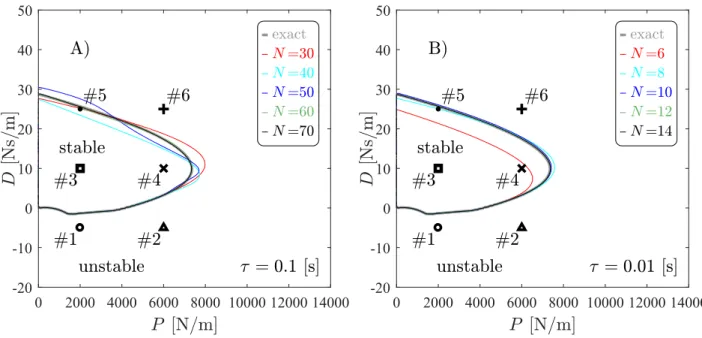
Figure 2: Stability diagrams, computed by the PT method, for the haptic system (60) without active human interaction (Ph = 0, Dh = 0) and with parameters given according to Table 1. In panels A) and B), stability boundaries are shown for two different time history lengths τ with increasing order N of polynomial approximation. The exact stability boundaries are shown with thick gray lines.
therefore the time length of history segment does not need to be equal to the human reaction delay τ. In this case, both the exact monodromy operator U and the exact stability boundary can be calculated (see Figures 2–3) as detailed in [25].
The results in Figure 2 show that in case of the PT method, the closer the length τ of history segment is to its minimum length τmin = ∆t, the smaller order N of polynomial approximation is required for accurate stability boundaries. Note that since (60) incorporates no time-periodic coefficients, there is no need for the piecewise constant approximation of time-periodic terms in case of the PT method. As a result, ˜v = 1 is applied during stability computations. Due to the lack of time-periodic coefficients, the principal period Tp =σ∆t can be chosen as an arbitrary integer σ ∈Z+ multiple of the sampling period ∆t. For the PT method σ= 1 was used, while for the SE method σ= 10 and σ = 20 were applied.
Figure 3 shows the stability boundaries computed by the SE method for different σ values, with changing orderN of polynomial approximation and with changing element numberE. In contrast with the PT method, the convergence rate of stability boundaries, in case of the SE method, depends not on the length of time history segment but on the length of the principle
0 2000 4000 6000 8000 10000 12000 14000 -20
-10 0 10 20 30 40 50
0 2000 4000 6000 8000 10000 12000 14000 -20
-10 0 10 20 30 40 50 0 2000 4000 6000 8000 10000 12000 14000 -20
-10 0 10 20 30 40 50
0 2000 4000 6000 8000 10000 12000 14000 -20
-10 0 10 20 30 40 50
Figure 3: Stability diagrams, computed by the SE method, for the haptic system (60) without active human interaction (Ph = 0, Dh = 0), with time history length τ = 0.1 [s] and system parameters given according to Table 1. In panels A) and B), stability boundaries are shown with fixed element number E and increasing order N of polynomial approximation for two different principal periods Tp = σ∆t . In panels C) and D), stability boundaries are shown with fixed order N of polynomial approximation and increasing E element number for two different principal periods. The exact stability boundaries are shown with thick gray lines.
period. As it can be inferred from Figure 3, longer principal period results slower convergence with respect to both the order N of polynomial approximation and element number E.
Figure 4 shows the stability boundaries computed by the PT and SE methods with non-zero human control parameters, that is with active human interaction. It can be observed that with the increase of order N of polynomial approximation, the stability boundaries converge to the same curve in case of both methods. As a reference, the case with no active human interaction is also plotted in Figure 4. It can be seen that the applied human control parameters affect the bottom part of the stability boundary, which corresponds to the experimental observations in [15].
Stability diagrams show only whether the system stays around its stationary state. However, it does not give insight into the decay of transients due to perturbations. In order to extract this
Figure 4: Stability diagrams, calculated by different numerical methods, for the haptic system (60) with active human interaction characterized by parametersτ = 0.1 [s], Ph =−200 [N/m], Dh = −5 [Ns/m] and by parameters given according to Table 1. The stability boundaries in panels A) and B) were computed with the PT and SE methods, respectively, in both cases for increasing order N of polynomial approximation. As reference, the exact stability boundary for the case of no active human interaction (Ph = 0, Dh = 0) is shown with gray color.
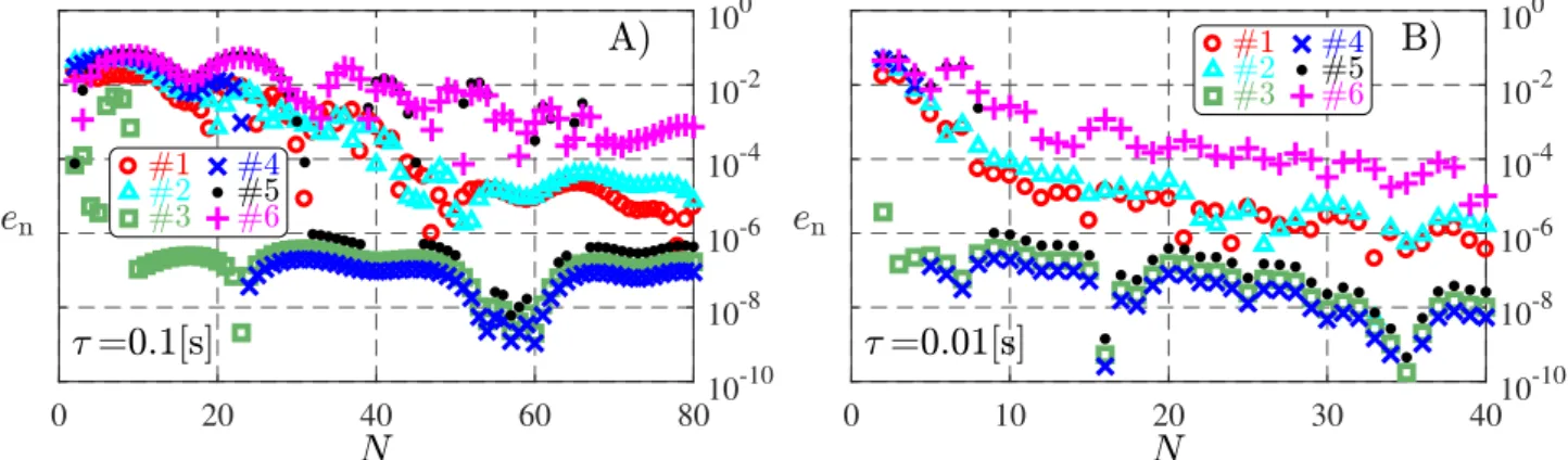
information one should determine the absolute value of the dominant characteristic multiplier (for further details see [13]). In Figures 5–7, the normalized error
en(k) =
µk−µ∗ µ∗
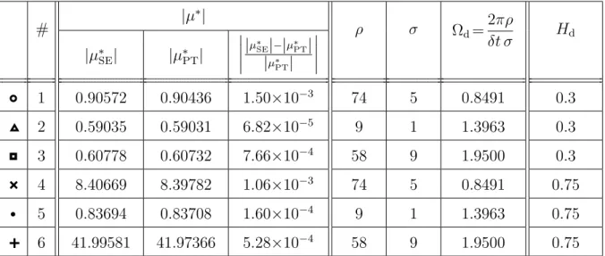
(61) of dominant characteristic multipliers µk with respect to the accurate dominant characteristic multiplier µ∗ is plotted in terms of approximation parameter k, in 6 points of the (P, D) parameter plane. The coordinates of these points, marked in Figures 2–4, are given in Table 2, where the absolute values of the accurate dominant multipliers employed for the construction of Figures 5–7 are shown as well. Note that only for the case without active human interaction force (that is whenPh= 0 and Dh = 0) can the exact dominant multiplierµ∗exactbe determined.
Otherwise the dominant multipliers can only be approximated. Consequently, in the case of non-zero active human interaction force (Ph=−200 [N/m] andDh=−5 [Ns/m]) the accurate dominant multipliers were calculated using the two different numerical schemes of Section 3 at high approximation numbers. In particular, for the pseudospectral tau method, the accurate dominant multiplier µ∗PT was computed using N = 80, while for the SE method, the accurate dominant multiplier µ∗SE was calculated using N = 80 and E = 1. As Table 2 and Figures 5–7 show, the absolute values of the dominant characteristic multipliers computed by the PT and SE methods converge to the same values in case of non-zero active human interaction force for all investigated points of control parameters with a normalized difference less than 0.1%.
Furthermore, both methods converge to the exact dominant multiplierµ∗exactin case of no active human interaction.
In conclusion, it seems likely that the presented methods give results convergent to the ex- act stability boundaries and dominant characteristic multipliers of (60) in the case of active human interaction. This convergence property might hold even for sets of system parameters different from those in Table 1. However, in order to verify this conjecture one must perform a
#
|µ∗|
P [N/m]
D [Ns/m]
(Ph, Dh) = (0,0) (Ph, Dh) = (−200,−5)[SI]
|µ∗exact| |µ∗SE| |µ∗PT|
|µ∗SE|−|µ∗PT|
|µ∗PT|
1 1.02382 1.02382 1.02382 5.39×10⁻⁶ 2000 -5
2 1.06473 1.06473 1.06472 8.13×10⁻⁶ 6000 -5
3 0.99877 0.99516 0.99516 2.87×10⁻⁷ 2000 10
4 0.99909 0.99760 0.99760 1.23×10⁻⁷ 6000 10
5 0.99749 0.99415 0.99317 9.82×10⁻⁴ 2000 25
6 1.05337 1.05343 1.05260 7.89×10⁻⁴ 6000 25
Table 2: Coordinates of the 6 investigated points of parameter plane (P, D), marked in Figures 2–4. The accurate dominant characteristic multiplier µ∗ is given by the exact dominant mul- tiplier µ∗exact for the case without active human interaction force (when Ph = 0 and Dh = 0) while it is given by the dominant characteristic multipliers µ∗SE and µ∗PT computed using the SE method with N = 80, E = 1 and the PT method with N = 80, respectively, and assuming active human interaction force (when Ph=−200 [N/m] andDh =−5 [Ns/m]).
precise theoretical convergence analysis, which is out of the scope of this paper. Nevertheless, the numerical results presented in this study can serve as a good base for a later theoretical convergence analysis.
0 20 40 60 80
10-10 10-8 10-6 10-4 10-2 100
0 10 20 30 40
10-10 10-8 10-6 10-4 10-2 100
Figure 5: Convergence diagrams of the dominant characteristic multiplier corresponding to the respective panels of Figure 2. The diagrams show the normalized error en of the dominant characteristic multiplier in terms of polynomial order N for 6 points of the (P, D) parameter plane given in Table 2 and indicated in Figure 2. Diagrams were computed by the PT method for the case of no active human interaction (Ph = 0, Dh = 0), using parameters according to Table 1 and τ = 0.1 [s] for panel A), and τ = 0.01 [s] for panel B).
4.2 Milling process with active damper
In machining processes the large amplitude self-excited vibration between the workpiece and the tool is called machine tool chatter. One of the most accepted explanations for machine tool chatter is the so called regenerative effect [1, 26], which can be modeled by DDEs. So-called
0 10 20 30 40 10-12 10-10 10-8 10-6 10-4 10-2 100
0 10 20 30 40
10-12 10-10 10-8 10-6 10-4 10-2 100
0 10 20 30 40
10-10 10-8 10-6 10-4 10-2 100
0 10 20 30 40
10-10 10-8 10-6 10-4 10-2 100
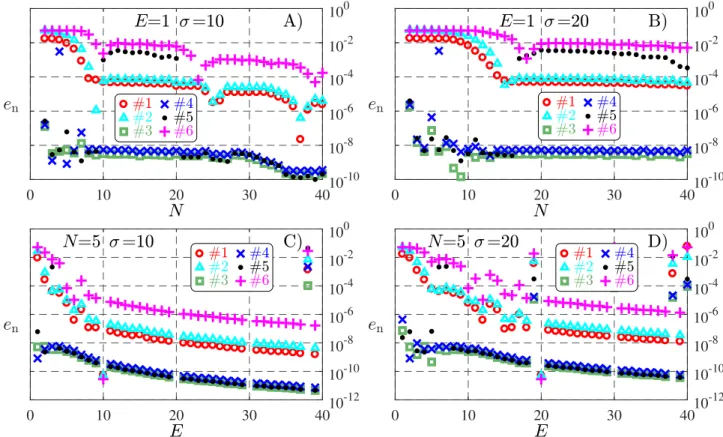
Figure 6: Convergence diagrams corresponding to the respective panels of Figure 3. The diagrams show the normalized error en of the dominant characteristic multiplier in terms of polynomial order N and element numberE for 6 points of the (P, D) parameter plane given in Table 2 and indicated in Figure 3. Diagrams were computed by the SE method for the case of no active human interaction (Ph = 0, Dh = 0) using parameters given in Table 1 and τ = 0.1 [s]. In panels A) and C)σ = 10, while in panels B) and D)σ = 20 is applied.
0 20 40 60 80
10-10 10-8 10-6 10-4 10-2 100
0 10 20 30 40
10-10 10-8 10-6 10-4 10-2 100
Figure 7: Convergence diagrams corresponding to the respective panels of Figure 4. Diagrams show the normalized error en of the dominant characteristic multiplier in terms of polynomial order N for 6 points of the (P, D) parameter plane given in Table 2 and indicated in Figure 4.
Panels A) and B) were computed by the PT and SE methods, respectively, using parameters given in Table 1 and assuming active human interaction characterized by parametersPh =−200 [N/m], Dh=−5 [Ns/m] and τ = 0.1 [s].
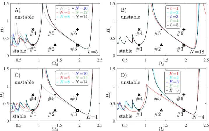
stability lobes diagrams (SLDs) are used to depict the regions associated with chatter-free machining in the parameter space of spindle speed Ω (in [rpm]) and axial depth of cut ap (see Figure 8). In the machining literature it has been a subject of great interest how the
stable domains in SLDs can be increased (thus chatter can be suppressed). There exist passive [27, 28], semi-active [29, 30] and active [31, 32] methods for the suppression of machine tool chatter. The active methods use a feedback loop, which usually involves a digital feedback controller in practice. However, apart from some studies presented for turning [33, 34], most existing models of active chatter suppression neglect the sampling effect and the zero-order hold of the feedback loop. Such study has not yet been presented for milling, mostly due to the required high computational effort of the stability analysis based on the existing standard methods of the literature. In this subsection, first a nonlinear mathematical model is derived for the milling process subjected to digital position control at the tool tip. Thereafter, stability analysis of the variational system around the stationary solution of this mathematical model is performed using the numerical methods detailed in Section 3 and results are visualized in the form of SLDs.
Figure 8: Model of milling subjected to active damping
One of the simplest models of regenerative vibrations in milling assumes that the tool (or the workpiece) can oscillate in the direction of the feed velocity only (for details see Chapter 5.2.1 in [8]). In addition, the model shown in Figure 8 takes into account a feedback loop controlled by a PD controller, which provides the active damping to the milling process. The displacement and the velocity of the tool tip are measured and used in the calculation of the control force Q which acts at the tool tip. The tool is modeled by a block of mass mt, connected to the tool holder via a spring of stiffness kt and a dash-pot of viscous damping bt as shown in Figure 8. The workpiece is assumed to move horizontally with a constant feed velocity vf relative to the tool holder. The undamped natural angular frequency of the tool is ωn = p
kt/mt and the damping ratio is ζ =bt/(2mtωn). Using dimensionless time ¯t = ωnt and dropping the bar immediately, the governing equations are
x(t) =˙ A0x(t) +C(x(tj−δt)−xd(tj−δt))−f(t,x(t),x(t−τd)), t ∈[tj, tj+δT), (62) with δt = ωn∆t and δT = ωn∆T being the dimensionless sampling and actuation periods, respectively. The state x(t) and the desired trajectory xd(t) are defined as
x(t) =
x(t)
˙ x(t)
, xd(t) =
xd(t)
˙ xd(t)
, (63)
while A0=
0 1
−1 −2ζ
, C=
0 0
−kP −kD
, f(t,x(t),x(t−τd)) =Fc(t,x(t),x(t−τd)) mtωn2
0 1
. (64) The controller uses PD control in order to stabilize the oscillator about the desired trajectory xd(t). The control forceQconsists of proportional and differential terms with feedback gainsP and D, respectively. Note that the difference between the measured and the desired trajectory is fed back with a delay δt in the control force term. This delay accounts for the processing time of the measured data and for the estimation of the desired state. Due to the rescaled time, dimensionless control gains are introduced as kP =P/(mtωn2) and kD =D/(mtωn). The dimensionless regenerative delay (which coincides with the tooth passing period) isτd = 2π/Ωd, with Ωd = 2πΩZ/(60ωn) being the dimensionless spindle speed and Z being the number of cutting teeth. The cutting force is the resultant of forces acting on the teeth (see Figure 9), hence the horizontal component of the resultant cutting force is
Fc(t,x(t),x(t−τd)) =
Z
X
p=1
gp(t) (Ft,p(t,x(t),x(t−τd)) cos(ϕp(t)) +Fn,p(t,x(t),x(t−τd)) sin(ϕp(t))), (65)
where the window function gp(t) =
(1 if ϕent ≤ϕp(t) mod 2π≤ϕex,
0 otherwise, (66)
models whether the pth tooth is in or out of cut while ϕent and ϕex stand for the entrance angle and the exit angle of the cutting teeth. For up-milling operation ϕent = 0 and ϕex = arccos(1−2ae/d), while for down-milling operationϕent = arccos(2ae/d−1) and ϕex =π, with ae being the radial immersion (see Figure 8) and d is the diameter of the tool (see Figure 9).
The tangential and normal force components of the pth tooth are both calculated according to
Figure 9: Cutting model: A) circular tooth path approximation B) tangential and normal cutting force components
![Figure 1: Concentrated parameter model of the haptic device based on [15] with simultaneous consideration of continuous delay τ in the human interaction and discrete delay ∆t in the digital controller.](https://thumb-eu.123doks.com/thumbv2/9dokorg/1407463.118522/11.892.178.706.307.573/concentrated-parameter-simultaneous-consideration-continuous-interaction-discrete-controller.webp)
![Figure 3: Stability diagrams, computed by the SE method, for the haptic system (60) without active human interaction (P h = 0, D h = 0), with time history length τ = 0.1 [s] and system parameters given according to Table 1](https://thumb-eu.123doks.com/thumbv2/9dokorg/1407463.118522/15.892.89.818.80.734/figure-stability-diagrams-computed-interaction-history-parameters-according.webp)
![Figure 4: Stability diagrams, calculated by different numerical methods, for the haptic system (60) with active human interaction characterized by parameters τ = 0.1 [s], P h = −200 [N/m], D h = −5 [Ns/m] and by parameters given according to Table 1](https://thumb-eu.123doks.com/thumbv2/9dokorg/1407463.118522/16.892.99.794.80.415/stability-calculated-different-numerical-interaction-characterized-parameters-parameters.webp)