Privacy-Preserving Release of Spatio-temporal Density

(1)

Density

Gergely Acs, Gergely Bicz´ok, and Claude Castelluccia

Abstract In today’s digital society, increasing amounts of contextually rich spatio- temporal information are collected and used, e.g., for knowledge-based decision making, research purposes, optimizing operational phases of city management, planning infrastructure networks, or developing timetables for public transportation with an increasingly autonomous vehicle fleet. At the same time, however, publishing or sharing spatio-temporal data, even in aggregated form, is not always viable owing to the danger of violating individuals’ privacy, along with the related legal and ethical repercussions. In this chapter, we review some fundamental approaches for anonymizing and releasing spatio-temporal density, i.e., the number of individuals visiting a given set of locations as a function of time. These approaches follow different privacy models providing different privacy guarantees as well as accuracy of the released anonymized data. We demonstrate some sanitization (anonymization) techniques with provable privacy guarantees by releasing the spatio-temporal density of Paris, in France. We conclude that, in order to achieve meaningful accuracy, the sanitization process has to be carefully customized to the application and public characteristics of the spatio-temporal data.

Gergely Acs

CrySyS Lab, Department of Networked Systems and Services, Budapest University of Technol- ogy and Economics (BME-HIT), Magyar tudosok korutja 2., 1117 Budapest, Hungary, e-mail:

acs@crysys.hu Gergely Bicz´ok

CrySyS Lab, Department of Networked Systems and Services, Budapest University of Technol- ogy and Economics (BME-HIT), Magyar tudosok korutja 2., 1117 Budapest, Hungary, e-mail:

biczok@crysys.hu Claude Castelluccia

INRIA, 655 Avenue de l’Europe, 38330 Montbonnot-Saint-Martin, France, e-mail:claude.

castelluccia@inria.fr

1

(2)

1 Introduction

Spatio-temporal, geo-referenced datasets are growing rapidly nowadays. With bil- lions of location-aware devices in use worldwide, the large scale collection of space- time trajectories of people produces gigantic mobility datasets. Such datasets are in- valuable for traffic and sustainable mobility management, or studying accessibility to services. Even more, they can help understand complex processes, such as the spread of viruses or how people exchange information, interact, and develop social interactions. While the benefits provided by these datasets are indisputable, their publishing or sharing is not always viable owing to the danger of violating individuals’ privacy, along with the related legal and ethical repercussions. This problem is socially relevant: companies and researchers are reluctant to publish any mobility data by fear of being held responsible for potential privacy breaches. This limits our ability to analyze such large datasets to derive information that could benefit the general public.

Unsurprisingly, personal mobility data reveals tremendous sensitive information about individuals’ behavioural patterns such as health life or religious/political be- liefs. Somewhat more surprisingly, such mobility data is also unique to individuals even in a relatively large population containing millions of users. For instance, only four spatio-temporal positions are enough to uniquely identify a user 95% of the times in a dataset of one and a half million users [13], even if the dataset is pseudonymized, i.e., identitifiers such as personal names, phone numbers, home ad- dress are suppressed. Moreover, the top 2 mostly visited locations of an individual is still unique with a probability of 10-50% [63] among millions of users. Notice that the most visited locations, such as home and working places, are easy to learn today from different social media where people often publicly reveal this seemingly harmless personal information. Therefore, publishing mobility datasets would put at risk our own privacy; if someone knows where we live and work could potentially find our record and learn all of our potentially sensitive location visits. Moreover, due to the large uniqueness of records, these datasets are regarded as personal information under several laws and regulations internationally, such as overall in the European Union. Therefore, their release prompt not only serious privacy concerns but also possible monetary penalties [18].

1.1 Privacy implications of aggregate location data

One might argue that publishing aggregate information, such as the number of individuals at a given location, is enough to reconstruct aggregate mobility patterns, and has no privacy implications. Indeed, aggregated information is usually related to large groups of individuals and is seemingly safe to disclose. However, this reason- ing is flawed as shown next. First, an attack is described that can reconstruct even entire individual trajectories from aggregate location data, if aggregates are periodically and sufficiently frequently published (e.g., in every half an hour). We also

(3)

illustrate the potential privacy threats of irregularly published aggregate location data, for example, when a querier (or the adversary) specifies the spatio-temporal points whose visits are then aggregated and released.

Consequently, aggregation per sedo not necessarily prevent privacy breaches, and we need additional countermeasures to guarantee privacy for individuals even in a dataset of aggregate mobility data such as spatio-temporal densities.

1.1.1 Reconstruction from periodically published aggregate data

The attack described in [61] successfully reconstructed more than 70% of 100 000 trajectories merely from the total number of visits at 8000 locations, which were published every half an hour over a whole week in a large city. The attack exploits three fundamental properties of location trajectories:

Predictability: The current location of an individual can be accurately predicated from his previous location because consecutively visited locations are usually geographically close. This implies that trajectories can be well-separated in space;

if two trajectories are far away in timet then they remain so in time(t+1)assuming thattandt+1 are not too distant in time.

Regularity: Most people visit very similar (or the same) locations every day. In- deed, human mobility is governed by daily routines and hence periodic. For example, people go to work/school and return home at almost the same time every day.

Uniqueness: Every person visits quite different locations than any other person even in a very large population, which has already been demonstrated by several studies. For example, any four locations of an individual trajectory are unique to that trajectory with a probability of more than 95% for one and a half million individuals [13].

The attack has three main phases. In the first phase, it reconstructs every trajectory within every single day by exploiting the predictability of trajectories. This is performed by finding an optimal match of locations between consecutive time slots, where geographically close locations are more likely to be matched. After the first phase, we have the daily fragments of every trajectory, but we do not know which fragments belong to the same trajectory. Hence, in the second phase, complete trajectories are reconstructed by identifying their daily fragments. This is feasible due to the regularity and uniqueness properties of trajectories, i.e. every trajectory has similar daily fragments which are also quite different from the fragments of other trajectories. Similarity of fragments can be measured by the frequency of visits per location within a fragment. Finally, in the last phase, re-identification of individuals are carried out by using the uniqueness property again; a few locations of any individual known from external sources (e.g., social media) will single out the individual’s trajectory [13]. As individual trajectories are regarded as personal data in several regulations internationally, the feasibility of this attack demonstrates that aggregate location data can also be regarded as personal data.

(4)

1.1.2 Reconstruction from irregularly published aggregate data

Another approach of releasing spatio-temporal density is to answer some counting queries executed on the location trajectories. The querier is interested in the number of people whose trajectories satisfy a specified condition (e.g., the number of trajectories which contain a certain hospital). Queries can be filtered instantly by an auditor, e.g. all queries which have too small support, say less thank(i.e., onlyk trajectories satisfy the condition), are simply refused to answer. However, this approach is not enough to prevent privacy breaches; if the support of two queries are both greater thank, their difference can still be 1. For instance, the first query may ask for the number of people who visited a hospital, and the second query for the number of people who visited the same hospital except locationsL₁andL₂. If the querier knows thatL₁andL₂are unique to John then it learns whether John visited the hospital.

Defenses against suchdifferencing attacksare not straightforward. For example, verifying whether the answers of two or more queries disclose any location visit can be computationally infeasible; if the query language is sufficiently complex there is no efficient algorithm to decide whether two queries constitute a differencing attack [30]. In Section 3.1, we show more principled techniques to recover individual location visits from the answers of a given query set.

1.2 Applications of spatio-temporal density

Spatio-temporal density data, albeit aggregated in nature, can enable a wide variety of optimization use cases by providing a form of location awareness, especially in the context of the Smart City concept [46]. Depending on both its spatial and temporal granularity, such data can be useful for optimizing the (i) design and/or (ii) operational phases of city management with regard to e.g., public transportation, local businesses or emergency preparedness. Obviously, spatial resolution determines the scale of such optimization, e.g., whether we can tell a prospective business owner to open her new cafe in a specific district or a specific street. On the other hand, it is the temporal granularity of density data that separates the application scenarios in terms of design and operational use cases.

In case of low temporal granularity (i.e., not more than a few data points per area per day), city officials can use the data for optimizing design tasks such as:

• planning infrastructure networks, such as new roads, railways or communication networks;

• advising on the location of new businesses such as retail, entertainment and food;

• developing timetables for public transportation;

• deploying hubs for urban logistics systems such as post, vehicle depos (e.g., for an urban bike rental system), electric vehicle chargers and even city maintenance personnel;

(5)

In case of high temporal granularity (i.e., several data points per area per hour) [33], spatio-temporal density data might enable on-the-fly operational optimization in the manner of:

• reacting to and forecasting traffic-related phenomena including traffic anomaly detection and re-routing;

• implementing adaptive public transportation timetables also with an increasingly autonomous vehicle fleet [52];

• scheduling maintenance work adaptively causing the least amount of disturbance to inhabitants;

• promoting energy efficiency by switching off unneeded electric equipment on- demand (cell towers, escalators, street lighting);

• location-aware emergency preparedness protocols in case of natural disasters or terrorist attacks [7].

These lists of application scenarios are not comprehensive. Interestingly, such an aggregated view on human mobility enables a large set of practical applications.

2 Privacy models

Privacy has a multitude of definitions, and thus different privacy models have been proposed. In terms of privacy guarantee, we distinguish between syntactic and semantic privacy models. Syntactic models focus on syntactic requirements of the anonymized data (e.g., each record should appear at leastktimes in the anonymized dataset) without any guarantee on what sensitive information the adversary can exactly learn about individuals. As opposed to this, semantic models¹ are con- cerned with the private information that can be inferred about individuals using the anonymized data as well as perhaps some prior (or background) knowledge about them. The commonality of all privacy models is the inherent trade-off between privacy and utility: guaranteeing any meaningful privacy requires the distortion of the original dataset which yields imprecise, coarse-grained knowledge even about the population as a whole. There is no free lunch: perfect privacy with maximally accurate anonymized data is impossible. Each model has different privacy guarantees and hence provide different accuracy of the (same) data.

1In our context, semantic privacy is not analogous to semantic security used in cryptography, where ciphertexts must not leak any information about plaintexts. Anonymized data (”ciphertext”) should allow partial information leakage about the original data (”plaintext”), otherwise any data release would be meaningless. Such partial leakage should include the release of useful population (and not individual specific) characteristics.

(6)

2.1 Syntactic privacy models

One of the most influential privacy model isk-anonymity, which was first introduced in computer science by [53], albeit the same notion had already existed before in statistical literature. In general, for location data,k-anonymity guarantees that any record is indistinguishable with respect to spatial and temporal information from at leastk−1 other records. Hence, an adversary who knows some attributes of an individual (such as few visited places) may not be able decide which record belongs to this person. Now, let us definek-anonymity more formally.

Definition 1 (k-anonymity [53]).LetP={P₁, . . . ,P|P|}be a set of public attributes, andS={S₁, . . . ,S|S|}be a set of sensitive attributes. A relational tableR(P,S)sat- isfiesk-anonymity iff, for each record inrinR, there are at leastk−1 other records inRwhich have the same public attribute values asr.

k-anonymity requires (syntactic) indistinguishability of every record in the dataset from at leastk−1 other records with respect to their public attributes. Orig- inally, public attributes included all (quasi)-identifiers of an individual (such as sex, ZIP code, birth date) which are easily learnable by an adversary, while the sensitive attribute value (e.g., salary, medical diagnosis, etc.) of any individual should not be disclosed. Importantly, the values of public attributes are likely to be unique to a person in a population [23], and hence can be used to link multiple records of the same individual across different datasets, if these datasets share common public attributes.

In the context of location data, where a spatio-temporal point(L,t)corresponds to a binary attribute whose value is 1 if the individual visited locationLat timetand 0 otherwise, such distinction of public and sensitive attributes is usually pointless.

Indeed, the same location can be insensitive to one person while sensitive to another one (e.g., a hospital may be an insensitive place for a doctor, who works there, and sensitive for a patient). Therefore, in a location dataset,k-anonymity should require that each record (trajectory) must be completely identical to at least k−1 other trajectories in the same dataset. Syntactically indistinguishable trajectories/records form a single anonymity group.

k-anonymity can be achieved by generalizing and/or suppressing the location visits of individuals in the anonymized dataset. Generalization can be performed by either forming clusters of similar trajectories, where each cluster has at leastktra- jectories, or by replacing the location and/or time information of trajectories with a less specific, but semantically consistent, one. For example, cities are represented by their county, whereas minutes or hours are represented by the time of day (morn- ing/afternoon/evening/night).

A relaxation ofk-anonymity, calledk^m-anonymity, was first proposed in [54].

This model imposes an explicit constraint on the background knowledge of the adversary, and requiresk-anonymity with respect to this specific knowledge. For example, if the adversary can learn at mostmlocation visits of an individual, then, for any set ofmlocation visits, there must be at least 0 orkrecords in the anonymized dataset which contain this particular set of visits. Formally:

(7)

Definition 2 (k^m-anonymity [54]).Given a datasetDwhere each record is subset of items from a universeU.Disk^m-anonymous iff for anymitems fromU there are 0 or at leastkrecords which contain these items.

In our context, universeU represents all spatio-temporal points, and an individual’s record has an item fromU if the corresponding spatio-temporal is visited by the individual.

No. Locations

1 {LA}

2 {LA, Seattle}

3 {NYC, Boston}

4 {NYC, Boston}

5 {LA, Seattle, NYC}

6 {LA, Seattle, NYC}

7 {LA, Seattle, NYC, Boston}

(a) Original

No. Locations 1 {West US}

2 {West US}

3 {NYC, Boston}

4 {NYC, Boston}

5 {LA, Seattle, West US}

(b) 2-anonymous

No. Locations

1 {LA}

2 {LA, Seattle}

3 {West US}

4 {West US}

(c) 2²-anonymous Table 1: Examples fork- andk^m-anonymity, where each row represents a record, public and sensitive attributes are not distinguished, and temporal information is omitted for simplicity. 2²-anonymity requires fewer generalizations and hence provides more accurate data at the cost of privacy.

If m equals the maximum number of location visits per record, then k^m- anonymity boils down to standardk-anonymity. However, the rationale behindk^m- anonymity is that the adversary is usually incapable of learning more than a few locations visits per individual (e.g., most people publicly reveal only their home and working places on social media, in which casem=2 if temporal data is dis- regarded). Clearly, requiring indistinguishability with respect to onlyminstead of all location visits of an individual requires less generalization and/or suppression thereby providing more accurate anonymized data. This is also illustrated in Table 1.

We must note that many more different syntactic privacy models (e.g.,`-diversity [39],t-closeness [37],(L,K,C)-privacy [42], etc.) have been proposed to mitigate the deficiencies ofk-anonymity. We refer the interested reader to [21] and [56] for more details on privacy models and their usage. In this chapter, we only consider syntactic anonymization schemes which rely onk- ork^m-anonymity.

2.2 Semantic privacy models

Most syntactic privacy models, such ask-anonymity, aim to mitigate only identity disclosure, when the adversary re-identifies a record in the dataset (i.e., infer the exact identity of the record owner). Although re-identification is clearly undesirable and explicitly addressed by most legal regulations worldwide, it is not a necessary

(8)

condition of privacy violations. That is, locating the anonymity group of a person (e.g., using his home and working places), the group itself can still leak a person’s visited places no matter how large the group is. For instance, each of thektrajectory may contain the same sensitive place, which means that the person also passed this place. The real culprit is the lack of uncertainty about the individuals’ presence in theanonymizeddataset; even a knowledgeable adversary, who may know that a person’s record is part of the original dataset, should not be able learn if this record was indeed used to generate the anonymized data. Another common pitfall of syntactic privacy models is the lack ofcomposability; the privacy of independent releases of the same or correlated datasets should not collapse but rather “degrade grace- fully”. However, this does not hold fork-anonymity: the composition ofk-anonym datasets, wherekcan be arbitrarily large, can only be 1-anonym (i.e., the anonymity guarantee completely collapses), which is also demonstrated in [22]. Composability is a natural requirement of any privacy model in the era of Big Data where many different pieces of personal data get anonymized and published about people by many different stakeholders independently. These different pieces may be gathered and combined by a knowledgeable adversary in order to breach individuals’ privacy.

Next, we present a model which addresses these concerns.

Intuitively, differential privacy [15] requires that the outcome of any computation be insensitive to the change of any single record inside and outside the dataset.

It allows a party to privately release a dataset: with perturbation mechanisms, a function of an input dataset is modified, prior to its release, so that any information which can discriminate a record from the rest of the dataset is bounded [16].

Definition 3 (Differential Privacy [16]). A privacy mechanism A guarantees (ε,δ)-differential privacy if for any databaseDandD⁰, differing on at most one record, and for any possible outputS⊆Range(A),

Pr[A(D)∈S]≤e^ε×Pr[A(D⁰)∈S] +δ or, equivalently, Pr_O∼_A_(D)h

log_Pr[A_(D)=O]

Pr[A(D⁰)=O]

>ε i≤δ.

Here,εis typically a modest value (i.e., less than 1), andδ is a negligible function of the number of records inD(i.e., less then 1/|D|) [16].

We highlight two consequences of the above definition which are often over- looked or misinterpreted. First, differential privacy guarantees plausible deniability to every individualinside as well as outsideof the dataset, as an adversary, provided with the output ofA, can draw almost the same conclusions about any individual no matter if this individual is included in the input ofA or not [16]. Specifically, Defi- nition 3 guarantees that every output of algorithmA is almost equally likely (up to ε) on datasets differing in a single record except with probability at mostδ. This implies thatevery possiblebinary inference (i.e., predicate) has almost the same probability to be true (false) on neighboring datasets [15]. For example, if an adversary can infer fromA(D)that an individual, say John, visited a hospital with probability 0.95, whereDexcludes John’s record, then the same adversary infers the same fromA(D⁰)with probability≈e^±ε×0.95+δ, whereD⁰=D∪ {John’s record}.

(9)

This holds foranyadversary and inference irrespective of the applied inference algorithm and prior (background) knowledge². That is, the privacy measureεandδ are “agnostic” to the adversarial background knowledge and inference algorithm.

Second, Definition 3does notprovide any guarantee about the (in)accuracy of any inference. There can be inferences (adversaries) which may predict the hospital visit of John quite accurately, e.g., by noticing that all records, which are very similar to John’s record (such as the records having the same age and profession as John), also visited a hospital [11], while other inferences may do a bad job of prediction as they cannot reliably sort out the records being similar (correlated) to John’s record. Definition 3 guarantees that the accuracy ofanyinferences, no matter how sensitive are, remain unchanged (up toε andδ) if John’s own record is included in the anonymized data. In other words, differential privacy allows to learn larger statistical trends in the dataset, even if these trends reveal perhaps sensitive information about each individual, and protects secrets about individuals which can only be revealed with their participation in the dataset³. Learning such trends (i.e., inferences which are generalizable to a larger population in interest) is the ultimate goal of any data release in general.

Therefore, the advantage of differential privacy, compared to the many other models proposed in the literature, is two-fold. First, it provides a formal and mea- surable privacy guarantee regardless what other background information or sophisticated inference technique the adversary uses even in the future. Second, following from Definition 3, it is closed with respect to sequential and parallel composition, i.e., the result of the sequential or parallel combination of two differential private algorithms is also differential private.

Theorem 1 ([40]).If each ofA1, . . . ,Ak is(ε,δ)-differential private, then their k- fold adaptive composition⁴is(kε,kδ)-differential private.

Composition property has particular importance in practice, since it does not only simplify the design of anonymization (sanitization) solutions, but also allows to measure differential privacy when a given dataset, or a set of correlated datasets, is anonymized (and released) several times, possibly by different entities.

There are a few ways to achieve DP and all of them are based on the randomiza- tion of a computation whose result ought to be released. Most of these techniques are composed of adding noise to the true output with zero mean and variance calibrated to desired privacy guarantee which is measured byε andδ. A fundamental concept of these techniques is theglobal sensitivityof the computation (function) [16]

whose result should be released:

2The inference algorithm and background knowledge influences only the probability of the con- clusion, which is 0.95 in the current example

3These secrets are theprivateinformation which discriminate the individual from the rest of the dataset and should be protected

4Adaptive composition means that the output ofAi−1is used as an input ofAi, that is, their executions are not necessarily independent except their coin tosses.

(10)

Definition 4 (Global L_p-sensitivity). For any function f : D → R^d, the L_p- sensitivity of fis∆_pf=max_D,D⁰||f(D)−f(D⁰)||_p, for allD,D⁰differing in at most one record, where|| · ||_pdenotes theL_p-norm.

The Gaussian Mechanism [16] consists of adding Gaussian noise to the true output of a function. In particular, for any function f : D→R^d, the mechanism is defined as G(D) = f(D) +hN1(0,σ), . . . ,Nd(0,σ)i, whereNi(0,σ)are i.i.d. normal random variables with zero mean and with probability density func- tiong(z|σ) = ^√¹

2π σ²e^−z²^/2σ². The varianceσ²is calibrated to theL2-sensitivity of f which is shown by the following theorem.

Theorem 2 ([16]).For any function f :D→R^d, the mechanismA A(D) = f(D) +hG1(σ), . . . ,Gd(σ)i

gives(ε,δ)-differential privacy for any ε<1 and σ²≥2(∆₂f)²ln(1.25/δ)/ε², whereGi(σ)are i.i.d Gaussian variables with varianceσ².

For example, if there ared possible locations and f returns the number of visits per location (i.e., the spatial density), then∆1f equals the maximum number of all visits of any single individualin any input dataset, where∆2f ≤∆1f. If∆2f is

“too” large orεand/orδ are “too” small, large noise is added providing less accurate visit counts. Also notice that the noise variance is calibrated to the worst-case contribution of any single individual to the output of f, which means that the count of popular locations visited by many individuals can be more accurately released than less popular locations with smaller counts. Indeed, all location counts are perturbed with the same magnitude of noise, hence the signal-to-noise ratio is higher for larger counts providing smaller relative error.

3 Releasing spatio-temporal data

Suppose a geographical region which is composed of a setLof locations visited byNindividuals over a time of interest withT discretized epochs⁵. These locations may represent a partitioning of the region (e.g., all districts of the metropolitan area of a city). The mobility datasetDofNusers is a binary data cube with sizeN· |L| ·T, whereDi,L,t=1 if individualivisited locationLin epochtotherwiseDi,L,t=0. That is, each individual’s record (or trajectory) is represented by a binary vector with size|L| ×T. The spatio-temporal density of locationsLis defined by the number of individuals who visited these locations as a function of time. More precisely, there is a time seriesX^L=hX₀^L,X₁^L, . . . ,X_T^L₋₁ifor any locationL∈L, whereX_t^L=∑^N_i=1Di,L,t

and 0≤t<T.X^Ldenotes the set of time series of all locationsLand is referred to as the spatio-temporal density of locationsLin the sequel.

5An epoch can be any time interval such as a second, a minute, an hour, etc.

(11)

In general, any data release is modelled by the execution of data queries. For example, if the querier is interested in the spatio-temporal density of locations S_L⊆L at time S_T ⊆ {0,1, . . . ,T−1}, then the query Q(S_L,S_T) is computed as Q(S_L,ST) =∑L∈S_L,t∈S_T∑^N_i=1Di,L,t=∑L∈S_L,t∈S_TX_t^L. This gives rise to at least three approaches for the privacy-preserving release of spatio-temporal density:

Approach 1: compute any queryQon the original dataD(orX^L) and release only the anonymized query result ˆQ(S_L,S_T);

Approach 2: anonymize the mobility datasetDinto ˆD, then release ˆDwhich can be used to answer any queryQas ˆQ(S_L,S_T) =∑L∈S_L,t∈S_T∑^N_i=1Dˆ_i,L,t;

Approach 3: compute the densityX^L from the original mobility dataDasX_t^L=

∑^N_i=1D_i,L,t, and release the anonymizedXˆ^L, whereXˆ^Lcan be used to answer any queryQ.

In Approach 1, a querier can adaptively (i.e., interactively) choose its queries depending on the result of previously answered queries. By contrast, in Approach 2 and 3, the released data are used to answer arbitrary number and type of queries non-interactively (i.e., the queries are independent of each other). In fact, Approach 1, 2 and 3 only differ in their adversary models: Approach 2 and 3 are instantia- tions of Approach 1 in the non-interactive setting where the possibly adversarial querier must fix all queries before learning any of its results. Specifically, Approach 2 is simply consists of answeringN· |L| ·T binary queries at once, where a query returns an element of the cubeD. Similarly, in Approach 2,|L·T|queries can represent the elements of every time series, where all queries are answered together. As detailed in the sequel, the decreased number of queries as well as the non-interactive answering mechanism is the reason that Approach 3 usually outperforms Approach 1 and 2 in practice as long as the only goal is to releaseX^Las accurately as possible meanwhile preserving the privacy of individuals. Hence, we will detail a specific solution of Approach 3 in Section 3.3 and briefly review the rest in Section 3.1 and 3.2.

3.1 Approach 1: Anonymization of specific query results

3.1.1 Syntactic anonymization

Privacy breaches may be alleviated by query auditing which requires to main- tain all released queries. The database receives a set of counting queries Q₁(S_L₁,S_T₁), . . . ,Q_n(S_L_n,S_T_n), and the auditor needs to decide whether the queries can be answered without revealing any single visit or not. Specifically, the goal is to prevent thefull disclosureof any single visit of any spatio-temporal point in the dataset.

Definition 5 (Full disclosure). D_i,L,t is fully disclosed by a query set {Q₁(S_L₁,S_T₁), . . . ,Q_n(S_L_n,S_T_n)}ifD_i,L,tcan be uniquely determined, i.e., in all pos-

(12)

sible data setsDconsistent with the answersc= (c₁, . . . ,c_n)to queriesQ₁, . . . ,Q_n, Di,L,tis the same.

As each query corresponds to a linear equation on location visits, the auditor can check whether any location visit can be uniquely determined by solving a system of linear equations specified by the queries. To ease notation, letx= (x₁, . . . ,x_N·|_L_|·T) denote the set of all location visits, i.e., there is a bijectionα:[1,N]×L×[1,T]→ [1,N· |L| ·T] such thatx_α(i,L,t)=Di,L,t. Let Q be a matrix withn rows and N·

|L| ·T columns. Each row inQcorresponds to a query, which is represented by a binary vector, indexing the visits that are covered by the query. The system of linear equations is described in matrix form asQx=c. Hence, the auditor checks whether anyxican be uniquely determined by solving the following system of equations:

Qx=c

subject to x_i∈ {0,1} for 1≤i≤N· |L| ·T (1) In general, this problem is coNP-hard as the variablesx_ihave boolean values [34].

However, there exists an efficient polynomial time algorithm in the special case when the queries are 1-dimensional, i.e. there is a permutation ofxwhere each query covers a subsequence of the permutation. Typical examples include range queries.

For instance, if locations are ordered according to their coordinates on a space-filling Hilbert curve, then range queries can ask for the total number of visits of locations (over all epochs) that are geographically also close. In the case of 1-dimensional queries, the auditor has to determine the integer solutions of the following system of equations and inequalities:

Qx⁰=c

subject to 0≤x⁰_i≤1 for 1≤i≤N· |L| ·T (2) Notice that the variables in Eq. (2) are no longer over boolean data and hence Eq. (2) can be solved in polynomial time with any LP solver [55]. The integer solutions of Eq. (2) equals the solutions of Eq. (1) for 1-dimensional location queries [34].

In the general case, when the queries are multi-dimensional, the auditor can also solve Eq. (2), and the final solutions are obtained by rounding: ˆx_i=1 ifx⁰_i>1/2 and

ˆ

x_i=0 otherwise. In that case, ˆx≈xfor sufficiently large number of queries [14].

In particular, if each query covers a visit with probability 1/2, thenO(|x|log²|x|) queries are sufficient to recover almost the wholex(i.e., datasetD). Even more, only

|x| number of deterministically chosen queries are enough to recover almost the entire original data [17]. In fact, these reconstruction techniques are the best known attacks against a database curator who answers only aggregate counting queries over boolean data.

Therefore, equipped with the original datax, the auditor can check whether any of the above attacks would be successful by comparingx with the reconstructed valuesˆx(orx⁰). If so, the auditor refuses to answer any of thenqueries.

The above query auditing techniques have several problems. First and foremost, refusing to answer a query itself can leak information about the underlying dataset

(13)

(i.e.,D) [44]. This would not be the case if refusal was independent of the underlying dataset (e.g., auditing is carried out without accessing the true answersc).

Second, they can be computationally expensive. Indeed, using the solver in [55] the worst-case running time isO(n|x|⁴)if|x| n. Finally, most query auditing schemes assume that the adversary has either no background knowledge about the data, or it is known to the auditor. These are impractical assumptions which is also demonstrated in Section 1.1.1, where the adversary reconstructed complete trajectories from aggregate location counts exploiting some inherent characteristics of human mobility.

3.1.2 Semantic anonymization

An alternative approach to query auditing perturbs each query result with some random noise and releases these noisy answers. In order to guarantee (ε,δ)- differential privacy, the added noise usually follows a Laplace or Gaussian distribution. If the noise is added independently to each query answer, then the error is O(p

nlog(1/δ)/εN)[16], whereNis the number of individuals andnis the number of queries. This follows from the advanced composition property of differential privacy [16]. Therefore, ˜Ω(N²)queries can be answered using this approach with non-trivial error (i.e., it is less than the magnitude of the answer). We note that at leastΩ(√

N)noise is needed per query in order to guarantee any reasonable notion of privacy [14, 16]. There also exist better techniques that add correlated noise to the answers. For instance, the private multiplicative weight mechanism [26] can answer exponentially many queries inNwith non-trivial error, where the added noise scales withO(p

log(T|L|)·log(1/δ)·log(n)/εN)^1/2.

In contrast to query auditing described in Section 3.1, the above mechanisms can answer queries in an on-line fashion (i.e., each query is answered as it arrives) and run in time poly(N,T|L|)per query. Moreover, the privacy guarantee is independent of the adversarial background knowledge (see Section 2.2). On the other hand, they distort (falsify) the data by perturbation, which may not be desirable in some practical applications of spatio-temporal density. Another drawback is that they are data agnostic and may not exploit some inherent correlation between query results which are due to the nature of the location data. For example, query results usually follow a publicly known periodic trend, and adding noise in the frequency domain can provide more accurate answers [5].

3.2 Approach 2: Anonymization of the mobility dataset

3.2.1 Syntactic anonymization

In general, anonymizing location trajectories (i.e., the whole cubeD) while preserving practically acceptable utility is challenging. This is due to the fact that loca-

(14)

tion data is typically high-dimensional and sparse, that is, any individual can visit a large number of different locations, but most of them typically visit only a few locations which are quite different per user. This has devastating effect on the utility of anonymized datasets: mostk-anonymization schemes generalize multiple trajectories into a single group (or cluster) and represent each trajectory with the centroid of their cluster [2, 43, 47]. Hence, every record becomes (syntactically) indistinguishable from other records within its cluster. This generalization is often implemented by some sophisticated clustering algorithm, where the most similar trajectories are grouped together with an additional (privacy) constraint: each cluster must contain at least ktrajectories. Unfortunately, such approaches fail to provide sufficiently useful anonymized datasets because of thecurse of dimensionality[6]: any trajectory exhibits almost identical similarity to any other trajectory in the dataset. This implies that the centroid of each cluster tend to be very dissimilar from the cluster members implying weak utility. Moreover, as the distribution of the number of visits of spatio-temporal points are typically heavy-tailed [45], projection to low dimen- sions and then clustering in low dimension also loses almost all information about the trajectories. This is illustrated by Figure 1 which shows the result of a state- of-the-art anonymization scheme, referred to as Never-Walk-Alone (NWA) [2], on a synthetic dataset with 1000 trajectories⁶. This scheme groupskco-localized trajectories within the same time period to form ak-anonymized aggregate trajectory, wherekwas set to 3 in our experiment and the greatest difference between any spatial point of two members of the same cluster is set to 2000 meters. Figure 1 shows that even with modest values ofk, the anonymized dataset provides quite imprecise spatial density of the city.

To improve utility while relaxing privacy requirements, k^m-anonymity has also been considered to anonymize location trajectories in [48]. However, most anonymization solutions guaranteeing k^m-anonymity has a computational cost which is exponential in min the worst-case, hence this approach is only feasible if mis small. This drawback is alleviated in [3], where a probabilistic relaxation of k^m-anonymity is proposed to release the location visits of individuals without temporal information. In theory, temporal data can also be released along with the location information if themitems are composed of pairs of spatial and temporal positions. However, care must be taken as the background knowledge of a realistic adversary cannot always be represented bymitems (e.g., it perhaps also knows the frequency ofmitems of a targeted individual).

Another approach improving onk-anonymization is p-confidentiality [10]; instead of grouping the trajectories, the underlying map is anonymized, i.e., points of interest are grouped together creating obfuscation areas around sensitive locations.

More precisely, given the path of a trajectory,pbounds the probability that the trajectory stops at a sensitive node in any group. Supposing that (i) the background knowledge of the adversary consists of stopping probabilities for each location in a single path and (ii) sensitive locations are pre-specified by data owners, groups of locations are formed in such a way that the parts of trajectories entering the groups

6 We used a subset of a larger synthetic trajectory dataset available on https://iapg.

jade-hs.de/personen/brinkhoff/generator/

(15)

Fig. 1: Never-Walk-Alone anonymization. Original dataset (city of Oldenburg in Germany) with 1000 trajectories (left) and its anonymized version (NWA from [2]) withk=3 where the distance between any points of two trajectories within the same cluster is at most 2000 meters (right). (Image courtesy of Gábor György Gulyás.)

do not increase the adversary’s belief in violating thep-confidentiality. Trajectories are then anonymized based on the above map anonymization. The efficiency and utility of this solution is promising, however, in cases where the adversarial background knowledge cannot be approximated well (or at all), semantic privacy models such as differential privacy is preferred.

3.2.2 Semantic anonymization

A more promising approach is to publish a synthetic (anonymized) mobility dataset resembling the original dataset as much as possible, while achieving provable guarantees w.r.t. the privacy of each individual. The records in both datasets follow similar underlying distributions, i.e., after modeling the generator distribution of the original dataset, random samples (records) are drawn from a noisy version of this distribution. A few solutions exist in literature where the generator distribution is modeled explicitly and noised to guarantee differential privacy. For example, DP- WHERE [41] adds noise to the set of empirical probability distributions which is derived from CDR (Call-Detail-Record) datasets, and samples from these distributions to generate synthetic CDRs which are differential private. Although this synthetic dataset can also be used to compute spatio-temporal density, it is usually not as accurate as perturbing the generator distribution of the spatio-temporal density exclusively [4]. Indeed, the accurate model of more complex data (such as the original mobility data) is also more complex in general (i.e., have larger number of parameters), which usually requires increased perturbation.

(16)

Some other works generate synthetic sequential data using more general data generating models such as different Markov models [9, 8, 29]. These approaches have wide applicability but they are usually not as accurate as a specific model tailored to thepublicly knowncharacteristics of the dataset to be anonymized. We illustrate this important point by the following example. DP-WHERE is designed for CDR datasets, and provides more accurate anonymized CDR data than a simple n-gram model [8]. For example, DP-WHERE models the distribution of commute distances per home location and then generates a pair of home and working places as follows. First, a home location is selected, which is followed by picking a distance from the (noisy) distribution of commute distances. Finally, a working place is selected which has this distance from the selected home location. This approach results in more accurate representation of home and working places than using the noisy occurrence counts of different pairs of home and working places like in [8].

This is because commute distances are modeled by an exponential distribution [41], and its single rate parameter can be estimated by the median of the empirical data (i.e., commute distances). Therefore, in DP-WHERE, the probability of a particular pair of home and working location depends on their distance, while in ann-gram model, it depends on the occurrence count of this pair in the original dataset. For instance, New York, as a home location, occurs equally likely with LA and Philadel- phia, as working places, in ann-gram model, if these pairs have the same frequency in the original dataset. By contrast, in DP-WHERE, New York is much more likely to co-occur with the geographically closer Philadelphia than with LA. The moral of the story is that achieving the best performance requires to find the most faithful model of the data whose accuracy does not degrade significantly due to additional perturbation.

3.3 Approach 3: Anonymization of spatio-temporal density

A simplek-anonymization of time seriesX^LreleasesX_t^L only ifX_t^L≥k. However, as it is detailed in Section 1, this still allows privacy violations through various reconstruction attacks. Hence, releasing spatio-temporal density with provable privacy guarantees, such as differential privacy, is preferred in many practical scenarios.

Within the literature of differential privacy, a plethora of techniques have been proposed to release 1- and 2-dimensional range queries (or histograms) while preserving differential privacy [59, 28, 49, 35, 38, 60, 12, 36, 5, 64, 62, 26] and they are also systematically compared in [27]. Indeed, interpreting query results (or bin counts in a histogram) as location counts, these techniques are directly applicable to release spatial density without temporal data. In theory, low-dimensional embed- ding, such as Locality-sensitive hashing (LSH) [50], may allow to use any of the above techniques to release spatio-temporal density.

Another line of research addresses the release of time series data with the guarantees of differential privacy. This is challenging as time series are large dimensional data whose global sensitivity is usually so large that the magnitude of the added

(17)

noise is greater than the actual counts of the series for stringent privacy requirement (i.e.,ε<1 andδ ≤1/|N|whereNis the number of records). Consequently, naively adding noise to each count of a time series often results in useless data. Sev- eral more sophisticated techniques [51, 31, 19] have been proposed to release time series data meanwhile guaranteeing differential privacy. Most of these methods re- duce the global sensitivity of the time series by using standard lossy compression techniques borrowed from signal processing such as sampling, low-pass filtering, Kalman filtering, and smoothing via averaging. The main idea that the utility degra- dation is decomposed into a reconstruction error, which is due to lossy compression, and a perturbation error, which is due to the injected Laplace or Gaussian noise to guarantee differential privacy. Although strongly compressed data is less accurate, it also requires less noise to be added to guarantee privacy. The goal is to find a good balance between compression and perturbation to minimize the total error.

There are only a few existing papers addressing the release of spatio-temporal density specifically. Although data sources (and hence the definition of spatio- temporal density) vary to a degree in these papers, the commonality is the usage of domain-specific knowledge, i.e., the correlation of data points at hand in both the spatial and the temporal dimension. This domain-specific knowledge helps over- come several challenges including high perturbation error, data sparsity in the spatial domain, and (in some of the cases) real-time data publication. In the context of releasing multi-location traffic aggregates, road network and density are utilized to model the auto-correlation of individual regions over time as well as correlation between neighboring regions [20]. Temporal estimation establishes an internal time series model for each individual cell and performs posterior estimation to improve the utility of the shared traffic aggregate per time stamp. Spatial estimation builds a spatial indexing structure to group similar cells together reducing the impact of data sparsity. All computations are lightweight enabling real-time data publishing.

Drawing on the notion ofw-event privacy [32], RescueDP studies the problem of the real-time release of population statistics per regions [57]. Suchw-event privacy protects each user’s mobility trace over any successivewtime stamp inside the infinite data grouping algorithm that dynamically aggregates sparse regions together. The criterion for regions to be grouped is that local population statistics should follow a similar trend. Finally, a practical scheme for releasing the spatio-temporal density of a large municipality based on a large CDR dataset is introduced in [4]. Owing to the complexity of its scenario and the innovative techniques used, we present this work in detail in Section 4.

4 A Case-study: Anonymizing the spatio-temporal density of Paris

In this section, we present an anonymization (or sanitization) technique in order to release the spatio-temporal density with provable privacy guarantees. Several opti- mizations are applied to boost accuracy: time series are compressed by sampling,

(18)

clustering and low-pass filtering. The distortion of the perturbation is attenuated via further optimization and post-processing algorithms. A striking demonstration shows that the achieved performance is high and can be practical in real-world applications: the spatio-temporal density of the city of Paris in France, covering roughly 2 million people over 105 km², is anonymized using the proposed approach.

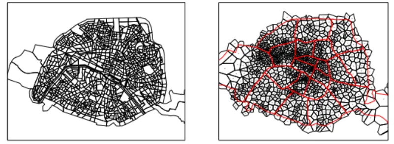
The specific goal is to release the spatio-temporal density of 989 non-overlapping areas in Paris, called IRIS cells. Each cell is defined by INSEE⁷and covers about 2000 inhabitants.Ldenotes the set of all IRIS cells henceforth, and are depicted in Figure 2 based on their contours⁸. We aim to release the number of all individuals who visited a specific IRIS cell in each hour over a whole week. Since human mobility trajectories exhibit a high degree of temporal and spatial regularity [24], one week long period should be sufficient for most practical applications. Therefore, we are interested in the time seriesX^L=hX₀^L,X₁^L, . . . ,X₁₆₇^L iof any IRIS cellL∈L, whereX_t^Ldenotes the number of individuals atLin the(t+1)th hour of the week, such that any single individual can visit a tower only once in an hour. We will omit tandLin the sequel, if they are unambiguous in the given context.X^Ldenotes the set of time series of all IRIS cells in the sequel.

To computeX^L, we use a CDR (Call Detail Record) dataset provided by a large telecom company. This CDR data contains the list of events of each subscriber (user) of the operator, where an event is composed of the location (GPS coordinate of the cell tower), along with a timestamp, where an incoming/outgoing call or message is sent to/from the individual. The dataset contains the events of N=1,992,846 users at 1303 towers within the administrative region of Paris (i.e., the union of all IRIS cells) over a single week (10/09/2007 - 17/09/2007). Within this interval, the average number of events per user is 13.55 with a standard deviation of 18.33 (assuming that an individual can visit any tower cell only once in an hour) and with a maximum at 732. Similarly to IRIS cells, we can create another set of time series X^C, whereX_t^Cdenotes the number of visits of towerCin the(t+1)th hour of the week.

To map the counts in X^C to X^L, we compute the Voronoi tessellation of the towers cellsCwhich is shown in Figure 2. Then, we calculate the count of each IRIS cell in each hour from the counts of its overlapping tower cells; each tower cell contributes with a count which is proportional to the size of the overlapping area.

More specifically, if an IRIS cellLoverlaps with tower cells{C₁,C₂, . . . ,C_c}, then X_t^L=

c

∑

i=1

X_t^Cⁱ×size(C_i∩L)

size(C_i) (3)

at timet.

The rationale behind this mapping is that users are usually registered at the geographically closest tower at any time. Notice that this mapping technique might

7National Institute of Statistics and Economics:http://www.insee.fr/fr/methodes/

default.asp?page=zonages/iris.htm

8Available on IGN’s website (National Geographic Institute):http://professionnels.

ign.fr/contoursiris

(19)

Fig. 2: IRIS cells of Paris (left) and Voronoi-tesselation of tower cells (right)

Algorithm 1Anonymization scheme

Input: X^T- input time series (from CDR), (ε,δ)-privacy parameters,L- IRIS cells,`- maximum visits per user

Output:Noisy time series ˆX^L

1: CreateX^Cby sampling at most`visits per user fromX^C 2: Compute the IRIS time seriesX^LfromX^Cusing Eq, (3) 3: PerturbX^Linto ˆX^L//see Algorithm 2

4: Apply smoothing on ˆX^L

sometimes be incorrect, since the real association of users and towers depends on several other factors such as signal strength or load-balancing. Nevertheless, without more details of the cellular network beyond the towers’ GPS position, there is not any better mapping technique.

4.1 Outline of the anonymization process

The aim is to transform the time series of all IRIS cellsX^Lto a sanitized versionXˆ^L such thatXˆ^Lsatisfies Definition 3. That is, the distribution ofXˆ^Lwill be insensitive (up toεandδ) to all the visits of any single user during the whole week, meanwhile the error betweenXˆ^LandX^Lis small.

The anonymization algorithm is sketched in Algorithm 1. First, the input dataset is pre-sampled such that only`visits are retained per user (Line 1). This ensures that the globalL₁-sensitivity of all the time series (i.e.,X^L) is no more than`. Then, the pre-sampled time series of each IRIS cell is computed from that of the tower cells using Voronoi-tesselation (Line 2), which is followed by the perturbation of the time series of all IRIS cells to guarantee privacy (Line 3). In order to mitigate the distortion of the previous steps, smoothing is applied on the perturbed time series as a post-processing step (Line 4).

(20)

4.2 Pre-sampling

To perturb the time series of all IRIS cells, we first compute their sensitivity, i.e.,

∆1(X^L). To this end, we first need to calculate the sensitivity of the time series of all tower cells, i.e.,∆1(X^C). Indeed, Eq. (3) does not change theL1-sensitivity of tower counts, and hence,∆1(X^C) =∆1(X^L).

∆1(X^C)is given by the maximumtotalnumber of (tower) visits of a single user inanyinput dataset. This upper bound must universally hold for all possible input datasets, and is usually on the order of few hundreds; recall that the maximum number of visits per user is 732 in our dataset. This would require excessive noise to be added in the perturbation phase. Instead, each record of any input dataset is truncated by considering at most one visit per hour for each user, and then at most` of such visits are selected per user uniformly at random over the whole week. This implies that a user can contribute with at most`to all the counts in total regardless of the input dataset, and hence, theL₁-sensitivity of the dataset always becomes`.

The pre-sampled dataset is denoted byX, and∆₁(X^C) =∆₁(X^L) =`.

In order to compute theL₂-sensitivity∆₂(X^L), observe that, for anyt, there is only a single tower whose count can change (by at most 1) by modifying a single user’s data. From Eq. (3), it follows that the total change of all IRIS cell counts is at most 1 at anyt, and hence ∆₂(X^L)≤∆₂(X^C) =√

` based on the definition of L₂-norm.

4.3 Perturbation

The time seriesX^Lcan be perturbed by addingG(p

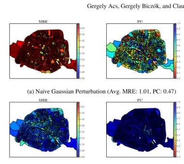
2`ln(1.25/δ)/ε)to each count in all time series (see Theorem 2) in order to guarantee(ε,δ)-DP. Unfortunately, this naive method provides very poor results as individual cells have much smaller counts than the magnitude of the injected noise; the standard deviation of the Gaus- sian noise is 95 withε=0.3 andδ =2·10⁻⁶, which is comparable to the mean count inX^L.

A better approach exploits (1) the similarity of geographically close time series, as well as (2) their periodic nature. In particular, nearby less populated cells are first clustered until their aggregated counts become sufficiently large to resist noise. The key observation is that the time series of close cells follow very similar trends, but their counts usually have different magnitudes. Hence, if we simply aggregate (i.e., sum up) all time series within such a cluster, the aggregated series will have a trend close to its individual components yet large enough counts to tolerate perturbation.

To this end, the time series of individual cells are first accurately approximated by normalizing their aggregated time series (i.e., the aggregated count of each hour is divided with the total number of visits inside the cluster), and then scaled back with the (noisy) total number of visits of individual cells.

(21)

Algorithm 2Perturbation

Input:Pre-sampled time seriesX^L, Privacy budgetε,δ, Sensitivity∆1(X^L) =` Output:Noisy time series ˆX^L

1: ˆSi:=∑_t=0¹⁶⁷X_tⁱ+G(2p

2`ln(2.5/δ)/ε)for eachi∈L 2: E:=Cluster(L,S)ˆ

3: foreach clusterE∈Edo

4: XÊ:=h∑_i∈EXⁱ₀,∑_i∈EXⁱ₁, . . . ,∑_i∈EXⁱ₁₆₇i 5: XˆÊ:=FourierPerturb(XÊ,ε/2,δ) 6: foreach celli∈Edo

7: Xˆⁱ:=Sî·(XˆÊ_t/||XˆÊ||1) 8: end for

9: end for

In order to guarantee differential privacy (DP), the aggregated time series are perturbed before normalization. To do so, their periodic nature is exploited and a Fourier-based perturbation scheme [51, 5] is applied: Gaussian noise is added to the Fourier coefficients of the aggregated time series, and all high-frequency components are removed that would be suppressed by the noise. Specifically, the low-frequency components (i.e., largest Fourier coefficients) are retained and perturbed with noiseG(p

2`ln(1.25/δ)/ε), while the high-frequency components are removed and padded with 0. As only (the noisy) low-frequency components are retained, this method preserves the main trends of the original data more faithfully than simply adding Gaussian noise toX^L, while guaranteeing the same(ε/2,δ/2- DP. Further details of this technique can be found in [4].

The whole perturbation process is summarized in Algorithm 2. First, the noisy total number of visits of each cell in L is computed by adding noise G(2p

2`ln(2.5/δ)/ε)to∑¹⁶⁷_t=0X_tⁱ for celli(Line 1). These noisy total counts are used to cluster similar cells in Line 2 by invoking any clustering algorithm aiming to create clusters with large aggregated counts overall (i.e., the sum of all cells’ time series within the cluster has large counts) using only the noisy total number of visits Sˆ_i as input. The outputE of this clustering algorithm is a partitioning of cellsL. When clustersEare created, their aggregated time series (i.e., the sum of all cells’

time series within the cluster) is perturbed with a Fourier-based perturbation scheme [5] in Line 5. Finally, the perturbed time series of each celliinLis computed in Line 7 by scaling back the normalized aggregated time series with the noisy total count celli(i.e., with ˆS_i). Since Line 1 guarantees(ε/2,δ/2)-DP to the total counts (∆₁(X^L) =√

`), it follows from Theorem 1 that Algorithm 2 is (ε,δ)-DP as the

Fourier perturbation of time-series is(ε/2,δ/2)-DP in Line 5 [4].