Theory for Proactive Operating Systems
D´aniel Krist´of Kiss∗† Andr´as R¨ovid‡
∗Doctoral School of Applied Informatics, ´Obuda University, Budapest, Hungary Email: kiss.kristof@phd.uni-obuda.hu
‡Institute of Intelligent Engineering Systems, ´Obuda University, Budapest, Hungary Email: rovid.andras@nik.uni-obuda.hu
†Mentor Graphics Corp. Montevideo utca 2/C, 1037 Budapest, Hungary, Email: daniel kiss@mentor.com
Abstract—The paper gives an overview of the current computer hardware trends and software issues. The optimal utilization of a multiprogrammed environment with multi-core processors is an extremely complex job. The scheduling in such an environment is an NP hard problem. The authors of the paper propose a novel approach to model the behaviour of the computing environment.
Furthermore an application modelling scheme is introduced. The proposed approach may allow the operating system to react to the changes in a reconfigurable environment. By using the introduced solution it would be possible to make the operating system more proactive.
I. INTRODUCTION
While computers become faster and smarter, the complexity of the software is growing rapidly. Here as computers first of all the personal computers, servers, tablets and smart phones are considered. Each of these cope with the same major problems which need to be solved. On one hand they consume relatively huge amount of energy, while on the other hand a portion of this energy is wasted due to running inefficient software.
It is well known that during the system lifetime the available resources are changing frequently. The software developers usually don’t know in advance how the resources used by their software will be scheduled. However this issue is strongly related to the overall performance of the system. The hardware configurations are different and changing, e.g. the servers can be reconfigured on the fly as well as the clock speed of the CPU may be changed while the software is running.
Mobile devices may change their own configuration according to the battery status or plan, as well. Computers may execute concurrently many applications sharing the same resources, such a way affecting the behaviour of the system as well as the behaviour of the applications. Changes in the capacity of the environment may be caused by software or hardware reasons. Software programmers may optimize their application code independently from the system resources which may be changed dynamically at runtime.
According to some researchers the applications may be implemented in a self-tuning or adaptive manner, such a way ensuring the adaptation of the software to the changes of the environment [1]. However this is rareness in the world of applications. For example a video encoding software may de- crease the precision to keep the required frame rate. Involving self-tuning mechanisms into more than one application may cause cross effects. Scalable applications are useful but cannot
Fig. 1. Scheduler without Intel Performance Counter Monitor[2]
Fig. 2. Scheduler using Intel Performance Counter Monitor[2]
solve the system wide problems and in some cases the appli- cation may interfere with the central control. Theoretically, the responsibility of the operating system is to provide a virtual environment for the applications.
Intel engineers published the result of their simulation [2]
of the scheduling. The simulation uses 1000 computation intensive and 1000 memory-bandwidth intensive tasks. Figure 1 shows the result of the simulation in case when the scheduler was not aware of the scheduled tasks. On the other hand Figure 2 shows the result when the scheduler was aware of the behaviour of tasks. The simulations show that such a scheduler executes the 2000 jobs 16% faster than a generic unaware scheduler on the test system. The measured speed-up is remarkable. In the simulation the tasks have been considered to have static behaviour, but this is not the case in the real word, i.e. each task may change is own behaviour. To use the performance counters in the scheduler effectively, the architecture and the parameters of the computer system, as well as the current and future behaviour of the tasks should be known.
The authors of the paper propose a modelling approach for modelling the behaviour of the computing environment.
Furthermore an application modelling scheme is introduced.
These models help us to analyse the system and to find its bottlenecks.
II. MODEL OF THE COMPUTER
Computing science started with one processor core per university, after switched to one processor per desktop. In the early 90‘s the server computers had more processors, and in 2002 the first processors with hyper threading technology have been released. That was a corollary of the Moore‘s law. They had to find a way to increase the computation capacity but the clock frequency could not been further increased because of the power dissipation limit of the silicon. That limit is called the power or thermal wall. The evolution of the processors is limited by three walls. The efficiency wall and the skew wall have also been reached. As a conclusion we cannot increase the computation capacity of a single core any more as we wanted to. In fact we could optimize the architecture, micro architecture and so on, but it would not bring reasonable increase in capacity. In 2006 Intel introduced the dual core CPUs. In 2011 Intel‘s current processors (the ”I family”) have 2-6 cores, each having hyper-threading capability [5]. Other manufacturer’s products have the same tendency. Without a deeper overview it is easy to recognize, that if we have a software, designed for a single core execution, we cannot buy a faster processor for faster computation. In 2007 Intel reported[8] the creation of a single chip with 80 computational units reaching 1.28 tera FLOPs. One of the most recent Intel research is the so called Single Chip Cloud computer. It contains 24 processing units and connections between them.
This architecture brings a new kind of constraints. It is important to note that some of the processors are dedicated to special activities, e.g. graphics or bus interface. The higher computation capacity comes from parallel processors[7]. This causes a radical change in the software design. From the software architecture point of view these architectures are challenging. Let us mention an other interesting example from the near past. As well known, hard disk drives are widely used for data storage. It was invented in 1956. In the last 50 years these devices are the dominant devices in the secondary storage area. This lead to the development of I/O schedulers in order to handle the seek time of devices and the rotational latency. In the last few years the solid-state drives became widely used, which are exceedingly different from the hard disk drives. New algorithms were and are still developed in order to support the SSDs. We can assume that the hardware changes have significant effect on the software both directly and indirectly.
In order to understand exactly these effects, the most suitable way is to create a mathematical model of the hardware architecture. With a proper model the analysis of the effects of the changes on the software may effectively be performed.
Furthermore it would be possible to model the behaviour of certain architectures and applied technologies which are not yet available, by modifying the suitable parameters of the developed model.
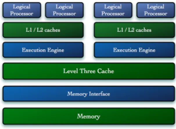
Fig. 3. Architecture of the Intel Core i7 processor
Two aspects are selected to describe the general model of a computer. The first part deals with the data access, i.e. it contains the capacity of the memories and the fetching de- pendency between the certain memory layers. The second part describes the computing capacity of the system, i.e. the hyper- threading support and internal communication speed in case of a Single Chip Cloud Computer. The computing capacity model contains the capacity of the computing elements together with the related restrictions. In this paper further elements, e.g. the input-output operations of the peripherals, etc. are not considered. However these elements may be modelled similarly.
The Data Access Model
The data access model describes the cost of data fetching and keeping it in memory.
Current computer architectures are built on multilevel trans- parent cache memories. The cost of the fetching of data always depends on the level it is held on. If a data block falls down the lower cache level, then next time it will be more cost-full to access it. The table I shows the state of the art memory access times.
Cache level Access time
1 L1 CACHE hit ˜4 cycles
2 L2 CACHE hit ˜10 cycles
3 L3 CACHE hit line unshared ˜40 cycles 4 L3 CACHE hit line shared
another core
˜65 cycles 5 L3 CACHE hit line modified
another core
˜75 cycles
6 remote L3 CACHE 100-300 cy-
cles TABLE I
CACHE ACCESS TIMES OF THEINTELCPUS[6]
The data access model implements arbitrary number of layers with different access properties in a flexible construc- tion. The granularity of the model shall be chosen wisely, i.e. the L1 cache is small and fast. It usually contains only 32k byte for data and 32k byte for program code while the
access time is around 4 clock cycles. This size enough only for the actual program code and some variables. Difference between the optimal L1 utilization and the average utilization is negligible small. Any system wide optimizer algorithm for the L1 utilization may consume much more computation time and resource then it could produce. Programers and the compiler could optimize the program code for better L1 cache utilization. We have chosen the L2 cache to be the first cache layer in the model.
Definition 1: fc(s) =ks|k∈R, s∈N is the cost function to fetchsamount of data from memory like device, where
1) k is constant time to reach one unit of data 2) sthe amount of required units of data
The access cost function is not always linear. A non-linear access cost function can be recognized when considering the hard-disk device. In this case the cost highly depends on the state of the hard disk, its internal cache size, state and the place of the data on the disk. In case of the SSD hard disks the cost function is totally different. This difference should be reflected on the disk-scheduling and related activities.
Definition 2: Ln is the nth memory layer access model.
MLn=hfc(s), Ciwhere 1) fc(s) is the cost function 2) C is the capacity of Ln layer
Today a common computer usually consists of a lot of memory layers with different properties, so our final model shall support any number of layers.
Definition 3 (Memory Access Model):
Mm = hML0, ML1, ..., MLni is the given memory access model. M stands for a vector of layers, where n represents the number of layers.
The Computing Model
The computing model describes the computation capacity of an arbitrary architecture. The capacity of a computation unit depends on the communication between the cores, the resources shared among the computation units and the nominal computing capacity.
Definition 4:
Mc =
C0,
Ic0,0, Ic0,1, ..., Ic0,n , ...,
Cn,
Icn,0, Icn,1, ..., Icn,n
is the ncored computer model where
1) Ica,b is the cost of notification between coreaandb 2) Cx is the nominal computing capacity of the corex A given computer may be described with theMm and the Mc pair.
III. APPLICATION CHARACTERIZATION
In this chapter we give an overview of the proposed appli- cation model. First of all the accuracy of the model shall be defined. In case of a too detailed model calculations would take to much time and also the model would consume significant amount of space. On the other hand a too simple model would make intolerable information lost and the connection between the model and the reality would be lost. From the
operating system point of view what the application does is not so important. The most important information for the scheduling is the resources need of the application. There are various kind of hardware resources. Some measurable parameters of the applications represent its requirements for resources. These parameters could be the followings: CPU usage, memory usage, I/O usage, disk usage, network usage, messages, number of threads etc. In the next sections we give a overview of the most important parameters.
Memory Usage Analysis
As well known the CPU is much faster than the memory.
The utilization of the CPU depends on the input data. Due to the fact that the memory stores the program code and the data, the memory is considered as the most sensitive resource.
In this paper the kernel side memory management will be considered. In all modern operating systems the programs are running in their own virtual memory space. The operating system manages the physical memory at a page level of granularity. As well known, by most platforms the program code is first loaded into memory before it can be executed.
The operating system keeps track on what data is required to reside in the memory.
Virtual memory is managed at a granularity of 4kB pages in OS X[3]. If during the address translation the affected page is not available in the memory, a page fault is generated. Page fault is handled by the operating system. When the system runs out of physical memory then pages are swapped out to the disk. It takes time to store and load pages from the disk which significantly decrease the performance, but increase the virtual memory size above the physical memory. The cost function of the memory operations are given in the previous chapter.
The ”work” necessary to keep track of pages and the physical memory is significant. For example when an application tries to allocate memory, the operating system has to find free regions in the physical memory and to allocate free pages.
When a page becomes inactive it may be swapped out to disk.
Later on if the page is requested again, then due to a pagefault it is loaded back into memory but probably it will be placed into a different location as previously. This phenomenon is called fragmentation.
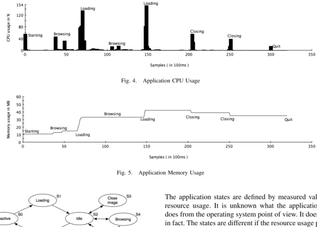
Let us to bring up and example. As a test application the Preview.app on MAC OS has been selected. This application can open pdf files or images and other file formats, as well. In this example we used two regular PDF files. Figure 5 shows the memory usage while in figure 4 the CPU usage can be followed. Note that the CPU usage could be more than 100%
because the usage is measured on each core separately. The test was executed on a MacBook Pro with Intel I5 quadcore CPU. In the figures different major activities can be followed.
The figure 6 shows the application states in a directed graph. Before theS1state the application is not activated. The probability of the transition from S0 to S1 is the frequency of the application launch. We can assume that the user may work with multiple documents simultaneously. The transition probability from the idle state to any other states depends on
Fig. 4. Application CPU Usage
Fig. 5. Application Memory Usage
Fig. 6. Application states
the application usage. The usage depends on the user. This is an important property of this solution.
Each state is described with a set of resource needs. The certain states may define a certain need. For example to start a program a predefined amount of RAM is needed to load the program code and allocate the global variables. For example when a new image is loaded then extra memory and CPU time are needed.
Definition 5: Letrstand for the resource and letarepresent the application. Let fra(t) be a continuous function which represents the usage in time of resourcer in the application a, i.e.fra(t)≥0.
fra0(t)is interpreted.
In practice the resource usage is calculated in sampling periods but here we consider continuous sampling. The function of the memory usage is not continuous. We consider that between two sample points the change is linear. The continuity of the function is a mathematical requirement.
Definition 6: LetR¯be a vector of the resource parameters.
The elements of this vector may correspond tof(tx)orf0(tx).
More detailed profiling is possible on the program code.
Profiling technologies are important in the nowadays devel- opment environments. In this paper these technologies are not detailed because each application is considered as a black box.
The application states are defined by measured values of the resource usage. It is unknown what the application actually does from the operating system point of view. It doesn’t matter in fact. The states are different if the resource usage parameters are different. The application does something different thinks while the resource usage parameters are same then the same state will be detected. Need of the states defined with some tolerance to reduce the number of the states. Letµis factor of this tolerance. We call state transition when the resource need is change.
Definition 7: LetS be a set of application states.
R¯s is the resource need of s. The si ∈ S is unique when µ∗R¯s∈ is not equal with any otherRs.
Definition 8: The probability of the state transitions P = S×S→R≥0.P is a Markov chain.
The behaviour of the application is defined by it’s Markov chain. Through the analysis of the chain information about the behaviour of the application and its and dependencies may be obtained. The execution of the application continuously updates its known states. Through the analysis of the Markov chain the resource needs of the application may be determined.
Theorem 1: If the current state of the application as well as its model is known then its future behaviour may be estimated with a given probability.
Theorem 2: The operating system allows to execute mul- tiple applications concurrently. If the current state of each currently running application together with their model is known then the future system load and behaviour may be estimated.
Resource need of the application usually depends on the usage. For example a web browser application may runs in multiple instance or uses multiple tabs. Some people prefer the multiple instance while others prefer multiple tabs. Resource need is different of the two cases. The introduced model
contains usage statistics indirectly which make predictions more reliable.
IV. FURTHERWORKS
In the current state of the research it is possible to build and analyse the Markov chains. The next milestone is to make actions according to the result of the model analysis. The current model describes the state without timing informations.
We are going to look for a method in order to add a timing attribute to the predictions as well as to analyse the term of predictions. The implementation of the measurement, analysis and decision making must be cost effective and fast operations.
We are going to check the possibilities of applying classical and soft computing techniques to solve the related problems.
V. CONCLUSION
In this paper a novel approach was introduced to model a computer environment and applications. The operating system has to know the actual hardware to make correct decisions.
Cost function of the operation could help the operating system to make optimal decisions. The proposed computer model may be an approach to determine these functions. Some examples are given to understand the model and the motivation behind it.
It is essential to understand the resource requirements of the software. The introduced modelling technique is based on the measurable parameters of the application. The created model gives a deep inside look into the application’s behaviour. The proposed model is based on Markov chains widely used not just in the information sciences. Based on the known model and the actual state of the application a prediction on its further behaviour and resource requirement may be performed. If the same technique is applied on each application then the future behaviour of the system may be predicted. Such application models let us to design more proactive operating systems.
ACKNOWLEDGMENT
The author(s) gratefully acknowledge the grant provided by the project TMOP-4.2.2/B-10/1-2010-0020, Support of the sci- entific training, workshops, and establish talent management system at the buda University.
REFERENCES
[1] Application Heartbeats: A Generic Interface for Specifying Program Performance and Goals in Autonomous Computing Environments, by Henry Hoffmann, Jonathan Eastep, Marco D. Santambrogio, Jason E.
Miller, and Anant Agarwal. The 7th IEEE/ACM International Conference on Autonomic Computing and Communications (ICAC2010), pp 79-88, June 2010.
[2] http://software.intel.com/en-us/articles/intel-performance-counter- monitor/ Visited February 2012
[3] https://developer.apple.com/library/mac/#documentation/Performance/
Conceptual/ManagingMemory/Articles/AboutMemory.html Visited February 2012.
[4] Kiss, D.K.; R¨ovid, A.; Multi-core processor needs from scheduling point of view, 8th International Symposium on Intelligent Systems and Informatics (SISY), vol., no., pp.219-224, 10-11 Sept. 2010
[5] Intel. Intel CoreTM i7-900 datasheet. s.l. : Intel, 2010.
[6] http://software.intel.com/sites/products/collateral/hpc/vtune/
performance analysis guide.pdf Visited February 2012
[7] Held, Jim, Bautista, Jerry and Koehl, Sean. From a Few Cores to Many:A Tera-scale Computing Research Overview. s.l. : Intel, 2006.
[8] Vangal, S.; Howard, J.; Ruhl, G.; Dighe, S.; Wilson, H.; Tschanz, J.;
Finan, D.; Iyer, P.; Singh, A.; Jacob, T.; Jain, S.; Venkataraman, S.;
Hoskote, Y.; Borkar, N.; , ”An 80-Tile 1.28TFLOPS Network-on-Chip in 65nm CMOS,” Solid-State Circuits Conference, 2007. ISSCC 2007.
Digest of Technical Papers. IEEE International , vol., no., pp.98-589, 11-15 Feb. 2007
![Fig. 2. Scheduler using Intel Performance Counter Monitor[2]](https://thumb-eu.123doks.com/thumbv2/9dokorg/1190749.87842/1.892.459.819.513.667/fig-scheduler-using-intel-performance-counter-monitor.webp)