CENTRAL RESEARCH INSTITUTE FOR PHYSICSBUDAPEST

(1)

G. F ORGÁCS A, ZAW A D O W S K I

KFKI-1977-7

GELL-MANN AND LOW ТУРЕ RENORMALIZATION GROUP AND THET>6 THEORY

H u n g a ria n ‘A cadem y o f S c ie n c e s

CENTRAL RESEARCH

INSTITUTE FOR PHYSICS

BUDAPEST

(2)

(3)

G E L L - M A N N AND L O W T Y P E R E N O R M A L I Z A T I O N G R O U P A N D T H E f 6 T H E O R Y

G. Forgács, A. Zawadowski Solid State Physics Department

Central Research Institute for Physics, Budapest, Hungary

Submitted to Journal of Physics

HU ISSN 0368-5330

(4)

Gell-Mann and Low renormalization group. Tricritical and critical properties in /or near/ three dimensions are discussed.

АННОТАЦИЯ

Исследовалась модель с помощью модифицированной ренормализацион- ной группы Гэлл-Манн и Ло. Обсуждаются критические и трикритические свойства модели при числе измерений три /или около трех/.

KIVONAT

A módosított Gell-Mann és Low féle renormalizációs csoport segítsé

gével megvizsgáljuk a cp6-os elméletet. Tárgyaljuk a kritikus és trikritikus tulajdonságait a modellnek 3 /vagy 3-hoz közeli/ dimenzióban.

(5)

Since Wilson's outstanding work /1974/ renormalization group technique has been widely used both in high energy physics and statistical mechanics. This method among others gave new insight into the problems of phase transitions/

anomalous dimensions/ asymptotic freedom etc. The term renormalization group is not new in physics and the best would be to speake of the revival of this approach. Renormal

ization group was succesfully used in quantum electrodynam

ics by Gell-Mann and Low /1954/ to describe ultraviolet and infrared properties of different vertex functions, Callan-Symanzik equation /197о / is also one of the possible formulations of the renormalization group. So,

renormalization group is neither new nor unique. Each of the above mentioned methods applied to the same problems/

gave the same results. But while the Gell-Mann and Low theory is tightly connected with perturbation theory /and the same is valid for the Callan-Symanzik equation/ the advantage of the Wilson's method is that in principle it can be formulated independently of the perturbation theory and in special cases concrete calculations can be performed without any reference to perturbation theory. Besides the

(6)

above mentioned methods there are others which can also deal with the problems of critical phenomena, such as Migdal's and Poljakov's bootstrap model /1968/, Abraham's and Tsuneto's sceleton graph expansion etc. In this paper we would like to further investigate the method first used by Sólyom /1973/. This method may be called as the combination of the Gell-Mann and Low and the Wilson method. In this context the following fact is very impor

tant. In the Wilson's case the underlying physics is quite clear, while in the Gell-Mann and Low approach one can not say that /at least not if statistical mechanical problems are investigated/. On the other hand, in our opinion, from mathematical point of view the latter method is much more tractable, since all the mathematics is contained in the Lie equations, characteristic of any continuous group. The advantages of both methods are contained in Sólyom's for

mulation of the renormalization group. More precisely it means that in this variant the cut-off transformation of Kadanoff is explicite, the mathematics is in the Lie equa

tions and the method is applicable to any renormalizable theory. At least the applications so far, such as to the

X

-ray absorbtion /Sólyom, 1974/, Kondo-problem /Sólyom, 1974/, one-dimensional electron systems /Menyhárd, Sólyom, 1973, Sólyom, 1973/, the calculation of anomalous dimensions /Forgács, 1974/, static critical phenomena /Forgács,

Sólyom, Zawadowski, 1976, referred to it in the following as FSZ,/ and dynamical critical phenomena /Greet, Zawadowski,

1975/ are consistent with this statement. The results in the case of the above listed applications were equivalent

(7)

to those obtained by different methods. However all these problems are so-called logarithmic that is if we let the physical cut-off in momentum space tend to infinity always

logarithmic divergencies would appeare. The relevant infra

red divergencies are also of logarithmic form. It would be good to know the limits of the applicability of this method, since it is extremely simple and physically very clear,

so if known exactly to what problems it can be applied, much work could be spared.

It is the aim of this paper to try to give an answer to the above question. For this reason we will very briefly describe the method /an extensive discussion of this method and also a comparison of it with the traditional Gell-Mann and Low theory is given in FSZ/, then apply it to a renormalizable, but not purely logarithmic problem /the

theory in d-3 dimension/. As a result we will obtain correct tricritical indices /correct to the calculated order/.

Then we will investigate ordinary critical phenomena at de3, and will see how the problem of strong coupling mani

fests itself in this approach. We will see, when comparing the results obtained by this method with those of the tradi

tional Gell-Mann and Low theory, that neither analytical method is better then the other or neither method is worse then the other in describing critical phenomena at d»3.

Nothing more definite can be said because of the strong coupling region.

(8)

2. The modified Gell-Mann and Low renormalization group

Let us assume that the Hamiltonian describes a renorma1izable theory. Let

tl - ' K » u lnt where

/

2

.

1

/

oc у

/

2

.

2

/

Here C\ are operators constructed out of the basic fields of the theory, are the coupling constants. We associate with each 0^ a vertex function I ^ s

' V <

I o k I ^/2.3/

In field theory < ? denotes vacuum expectation value, in statistical mechanics it is the statistical average. The

Г ^ are defined in such a way that in the zeroeth order of the perturbation theory all are equal to unity. If there are П basic fields in the theory, there will be n prop

agators

G, /GJil ■ ■ • C-n‘

Introducing a cut-off

A

in mo

mentum space, we assume the following invariance properties to be valid:

G s л)* G s (p) mp, / л I

* 4 ' A

/2 .6/

Here m. are the renormalized masses /mass renormali

zation is performed on mass shell; see below for a specific model/

(9)

£ ( z s Z h ) is a product of a certain number of -Z”5 and one . The explicite form of the ^ function is

constructed in such a way that the following relations hold:

**G*s(fz , nQ^j.k A)^**

Zt rt П G ^ U /П •

Q } - le. t x "

where * ; Л.о is the number of the incoming lines

s-1 1

in the ^ - t h vertex. Note that the 2 SlZ ^ factors can be expressed by I ^ and Q ^ from equations /2.4/ and /2.5/, so the ^ function can also be written in terms of Z S,Zk • What do the invariance equations mean? They mean /if they are valid/ that for the matrix elements of the S-matrix of the field theory /in statistical mechanics the analogue of the S matrix is the partition function/

<9 5

с)

л

⁵^/|

^ s .

L-I Зек^ 5c/ - = о /2.8/

where the changes are consistent with /2,6/. It is assumed that the *LjZk factors are functions only of and , but are independent of the momenta and masses.

We can prove the validity of these transformations only a posteriory by the help of the perturbation theory. In all the so far applications it turned out that the transfor

mations /2,4/ - /2.6/along with /2.7/ could be built up explicitely.

Introducing dimensionless coupling constants, and di

mensionless functions C-\= —Ci / G ó are the bare propagators/,after eliminating the 'Z factors, equations /2.4 - 2.6/ can be cast into differential form:

(10)

A can be any of the 0/5 Гь functions. Неге И/ - V, • v *fn'/

■> p J ^ / -J

Г _ ✓yO

X- / are dimensionless coupling constants,

C/f(v, Ugj are called invariant coupling constants, /defined later for a specific model/, the transformations /2.4 -2.6/

leave them invariant.

The equations /2.9/ are the Lie equations of the renormali

zation group. These equations do not determine uniquely the A functions. /Bogoljubov and Shirkov, 1973/ In the general

solution arbitrary functions of several variables appear.

Therefore what one can do is calculating the right hand sides by the help of perturbation theory and then solving the equa

tions; in this way improving the results of the perturbational calculat ions.

3. The G theory

Let our Hamiltonian be in dimensional space

/It is actually the Hamiltonian devided by ^ / , where k is the Boltzmann constant, I is the temperature./ This corresponds

/2.1о/

to

/3.2/

(11)

in the previous section, but actually all the propagators are equal and we call it

G

^. Let us perform mass renormal

ization in such a way that

t - m z- О

/ з . з /

The statistical mechanical analogue of m is the coherence length у , namely

m = f

^/3.4/

It means m disappears on the critical line. The equations corresponding to /2,4 - 2.6/, expressed via dimensionless quantities, are

i } ~ I

^ G Here

c;^ ( Л г' 7? "Л, 4 4 (''/ч,, U6) ,

Г} С л 1 ы ‘ ('fr-UvWj /7 6fr- Ч /

~‘, = u "

t i - t i /4L -?</ т / /|г 1/ '

( Л , tu,,т )

“(£)*

Ч - 4

с М

Л' 4<J~<o

/3.5/

/З.б/

/3.7/

/3.8/

/3.9/

3.1о/

are dimensionless coupling constants. For simplicity we choose the external momenta of the vertex functions in such a way that they depend only on a single external momenta variable. We

now try to determine the Z-L factors to first order in the coupling constants. The invariant coupling constants C ^ j ^ G )

~ ~ ~z г

are Ц, and U b with A replaced by either & or ^ . Since finally we will be interested in the tricritical /or

(12)

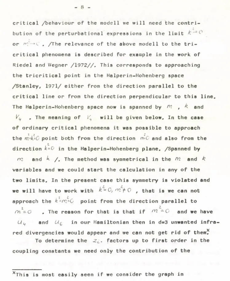
critical /behaviour of the modell we will need the contri

or . /The relevance of the above modell to the tricritical phenomena is described for example in the work of Riedel and Wegner /1972//, This corresponds to approaching the tricritical point in the Halperin-Hohenberg space

/Stanley, 1971/ either from the direction parallel to the

critical line or from the direction perpendicular to this line.

The Halperin-Hohenberg space now is spanned by /Т! , к and K, . The meaning of V4 will be given below. In the case of ordinary critical phenomena it was possible to approach

г г i

the m zk=C point both from the direction n^C and also from the direction k-0 in the Halperin-Hohenberg plane. /Spanned by

rrz and k /. The method was symmetrical in the />2 and k variables and we could start the calculation in any of the two limits. In the present case this symmetry is violated and we will have to work with k = C, m + Q t that is we can not

■ г l

approach the k=m.^C point from the direction parallel to

г l

Гп. — o , The reason for that is that if ^ — G and we have U L, and in our Hamiltonian then in d=3 unwanted infrared divergencies would appear and we can not get rid of them.

To determine the factors up to first order in the coupling constants we need only the contribution of the

xThis is most easily seen if we consider the graph in

figure 1. This graph will give contribution to the d function.

The analytic expression for this graph is

If CLP is finite anc/ /7?^ then this integral is infrared divergent.

bution of the perturbationa1 expressions in the limit к

(13)

graphs in figure a. /We do not have to calculate the d function, since because of the mass renormalization /3.3/

it does not give any contribution in the first order./

Since now fc — Q t the analytic expressions for the graphs a and b are proportional to In , and for the graphs c and d to — . Note that we keep all infrared diver-

no

gent contributions. ~he cross in figure 2 means that since in the graph calculation the I^ vertex always appears with the coupling constant Uu t U r J O - -1— /to first order

in Uq,/, therefore instead of у we can introduce this combination as a coupling constant. We call this new coup

ling constant Y^ . The analytic expressions for 7 and

Г

^q are

Г = it uc lu. — ' - y Í -г* {— )' -11 / З Л 1 /

1 Ч Э Ю ж 1 ° / I 2- JZrJ ^ L 4 ( / I / 4 ,

Г - i t 3^ r2 -L /, J m l _ ^4tN ,f j Jj t- / m ) .7 /3 12/

From the point of view of our theory the introduction of Y^ is crucial. If we use the original coupling constants and try to determine the factors in the equations /3.5 - 3.7/ it turns out that there are no such ^ /depending only on and % / with which we can satisfy these equa

tions. If instead of we write /3.8/ for , the equa

tions can be shown to be valid and the ZL factors are

2

1

-It

^U /

Л1

^-

A><p

^{I '}

I

^/

л 7

, , ,

•* ' л * - И Р * ч ( л ) -'J, / З Л З /

7,4 « ,it л а й

^,

a - jail

^r

\

° ^/1г Gj L '1( a ) 7 /3.14/

In the language of Riedel /1972/ it means that the proper scaling field besides rri is not <7 but ^ /Riedel and Wegner 1972/.

(14)

After having determined the Z.'L factors the Lie equations

r\ p

for I'* and U can be set up. They are

d — J -L Jl lHL t y* 7

СЧ У 4 L Я & 3 2 0 й г * 4Л /г3- -J /3.15/

- j L t,« r 4 * J-Z + 3/V « Л 7 У У 7

^ Y G / 6 / З Л 6 /

2

Here </ - — г / £ = 3 - d /VVe are performing the calculation in 3-d dimension in order to get a non-trivial fix point for

4? /.

Before analyzing the above equations let us write down

the expressions for , I and also the equations correspond

ing to /3.15/ and /3.16/ in the traditional Gell-Mann and Low theory. We do not want to describe this method here, since it can be found in many places /for example Bogoljubov and

Shirkov, 1973; in connection with critical phenomena see also the work of Di Castro /1972/ and FSZ./, Let us mention only that in this approach the exact invariance property of the

perturbation series is used to introduce multiplicative factors, which permit a suitable normalization for the Green's functions and vertex functions. Because of this normalization the vertex

functions are not those given by /3.11/ and /3.12/. Denoting the normalized vertex functions by ' ^ and / & , they can be written as

1 4 + A’ ~ / / = -/ ■+ ---- U / ,

H J i o / 6

$ t /V ~

4 * 4 ( * * - < ) . 1 6 * *

an*..3/v

(7 /. ~ -vvt/v■ ~ / ~ ,)

; 1 3 ' “ T i “ У I У ' У

/ з . 17/

/3.18/

(15)

Here

Г а “ '

^{^ ~} ^{< V}^j^Í^t ⁵ ^6/^ь^, ^{и ч}^a^{^ ч} ^{cj-'t ^}^, <Л, = °C /^{-tci- G} and Д is connected with the normalization of /

'X'

Г , In the above we adopted the normalization

and

/

\($ч)'Гл (9ч)-1

^/3.19/

Details concerning the normalization problem can be found in FSZ, Note that the and ГТ ( L = written in terms of the appropriate variables differ only in the coefficients of the 4 -point contributions, but this is true only in first order. In higher order calculation the coefficients in front of the logarithms also may be different /see FSZ/. In the case of the Gell-Mann and Low theory for the Lie equations of the

Г У

invariant coupling constants one needs ' i, and ' G /and not and /. The Lie equations now are

а к й(ч) /

I ^ ^

Ы Ч У о/ йе * (5)

Ы У

;í- Ь V i

J- t и * <Рм/ 7

L t U

6 V

Vd'O - *■

, I

4 w<? J

/3.20/

/3.21/

1Ü * ■ L,<?

Let us anal ize equations /3.15/, /3.16/ and /3.2о/, /3.21/.

L ( s) = сл

S

^

r

u *

/3.24/

with

/ / 3 ( t/v)

^ - ЗГ ’ - ^ 7 /3-25/

(16)

/» p

either U c' or UG" and 5 is either у or t( . Since w <0 the fix point /3.22/ can be stable only if c ( = 0, But К

/the bare or 1'^ /, therefore

с , « К

, so

C , - C

implies / - C . On the other hand we argued that h) is a scaling field, therefore the fix point /3,22/, together with ft - О is the tricritical fix point. /The tricritical fix point is the one, where n V - A - C /

Let us see how to calculate tricritical indeces in this formalism. As an example we will calculate the tricritical £ indece, the definition of which is

*?

d /at the tricritical point/ ■"— ' h. /3,26/

k -»о

Being at the tricritical point means К ~ О and we have a purely logarithmic problem. As it was shown in FSZ in such a case

Л е ю . L ( m ~D; k.) — ю\ L. k-oj /3.27/

о m ^ > 0

This means we can use the expression /3.22/ for for the determination of ^ *

To find the o| function we calculate the right hand side of the corresponding Lie equation to second order in L , that is we calculate the contribution of the graph in figure 4, The solution of the Lie equation is

where

о/ ~ C & ) t-> о

/3.28/

r-

^/3.29/

(17)

From the definition of ю and 5 we finally get

L 1 6 7 (З Ы + I Z )x /3.30/

This result is in agreement with earlier calculations /Stephen and MeCauley, 1973/. Since in the result only S and

appear it is clear that both the cut-off scaling version of the multiplicative renormalization group and the Gell-Mann and Low theory give the same result. This is an other confirmation of the equivalence of the two methods in the case of logarithmic problems. Corrections to the above scaling behaviour can be obtained in the way similar to that described in detail in FSZ.

B. The tricritical region with К Ф 0 .

Let us see what happens if К has a small positive value. In this case the trajectories in figure 3 will be nearly parallel to K - O , to same value of S and then will bend and tend to another fix point. Unless the n (~ ^ °r 4 / term in equa

tions /3.15/, /3.16/ and /3.26/, /3.21/ can be neglected in comparison to the lS' term we will have the same behaviour as before. For that we need /in d=3/

«

L R

^/3.31/

For the bare coupling constants К and L the condition /3.31/

means that in the lowest order

L

^« ¹

/3.32/

This is the same relation used by Stephen et al, /1975/,

but here /3.32/ is the trivial consequence of the Lie equations and we do not have to start with this condition. If

(18)

iC с ‘/г /

Ь ~ we get the border-line between the tricritical and critical regions /figure 3/ with the crossover exponent ^ /Amit and De Dominicis, 1973; Riedel and Wegner, 1972/.

C. Critical phenomenal at d=3.

When /3.32/ is replaced by

“ Й < < A > j L < < 1 /3.33/

we are out of the tricritical region, but still may use per

turbation theory to construct the right hand sides of the Lie equations. However we lose the logarithmic nature of the problem and simultaneously see that the fix point now is out

side of the weak coupling region. The right-hand sides of the Lie equations calculated to any finite order in perturbation theory can be used only in a very narrow region of the 'S4 variable /Wohrer and Brezin, 1976/. The dashed trajectories are just qualitative lines and show only the trend of the changes. The same is valid for the trajectories on the L - O

line since in this case also an C(<) fix point would occur in the lowest order. So, in the critical domain in the case d=3, the Lie equations are valid only in a very narrow region and we can not trace the behaviour of the system up to the critical point.

4 Conclusions

We investigated the theory near d»3 in the frame

work of two different formulations of the multiplicative re

normalization group. We saw that as in the previous works

(19)

there is no difference between the two versions unless we deal with a purely logarithmic problem ( 6 -C), What is new in our analysis is that even when the у 4 coupling is considered

and the theory loses its logarithmic character, the invariance equations /3.5/ - /3.9/ still can be constructed with the jz: factors depending only on the coupling constants and the ratio

./Although the ^ factors have been calculated only up to first order it is not very difficult to show that the above i8 valid also in higher orders./ While in the case of

logarithmic problems we could compare the two theories numer

ically, it can not be done here, since in order to calculate critical indecee in d=3 we have to cross the border-line between the weak and strong coupling region and therefore the numerical values obtained in such a way for critical indeces should not be taken too seriously. /They are as bad or as good as indeces obtained by putting £-1 in the calculations around four di

mensions./ However we may conjecture that in all cases /that is not only in the case of logarithmic problems/ when we have scaling in our theory, with appropriate normalization for the vertex functions in the Gell-Mann and Low theory the two methods are equivalent. When there is no scaling the cut-off version can not be used while the original Gell-Mann and Low theory, still works but does not improve the results of the perturba- t iona 1 ca leu lat ion. If the scaling is approximate the j r

factors can be calculated approximately and again there is no difference between the two methods /Iche, 1973/.

(20)

Acknowledgments

The authors are indebted to □ . Sólyom for valuable discuss ions.

(21)

Figure 1.Infrared divergent graph in the case m *02 . Figure 2.Graphs giving contributions to the vertex funct ions.

Figure 3.Trajector ies of the Lie equations.Reg ion 1 is the tricritical region.In region 2 perturbation theory still can be used to construct the right hand sides of the Lie equations.Region 3 is the strong coupling region.The dashed trajectories show only the trend of the changes.

Figure 4.The graph giving contribution to the tricritical

Y) indece in the lowest order.

»

Ф

(22)

Abrahams E. and Tsuneto T. 1973 Phys.Rev.Lett. 3o, 217 Amit D.3. and De Dominicis C.T. 1973 Phys.Lett. 45A, 193 Bogoljubov N.N. and Shirkov D.V. Introduction to the Theory

of Quantized Fields, Interscience Publ.London,1959 Brezin E., Le Guillon 3.C. and Zinn-Oustin 3. 1973 Phys.Rev.

D8, 434 Callan C.G. l97o Phys.Rev. D2, 1541

Di Castro C. 1972 Lett. Nuovo Cimento 5, 69 Forgács G. 1974 Lett. Nuovo Cimento JL2, 845

Forgács G., Sólyom 0. and Zawadowski A., 1976, to be published Fowler M., Zawadowski A., 1971 Solid St.Commun. 9, 471

Gell-Mann M, and Low F.E. 1954 Phys.Rev. 95, l3oo Greet G, and Zawadowski A., unpublished

Iche G. 1973 3. Low Temp, Phys. JJ., 215

Menyhárd N., Sólyom 3., 1973 3. Low Temp.Phys. 12, 529 Migdal A.A. 1968 Zh.E.T.F. 55, 964

Poljakov A.M. 1968 Zh.E.T.F. 55, lo25 Riedel E.K., 1972 Phys.Rev.Lett. 28, 675

Stanley H. E,, Introduction to Phase Transitions and Critical Phenomena, Oxford, 1971

Stephen M.3., Abrahams E,, Straley 3.P., 1975 Phys.Rev.B12, 256 Sólyom 3., Zawadowski A,, 1974 3,Phys. F. 4, 8o

Sólyom 3. 1973 3. Low Temp. Phys. 12, 547 Sólyom 3. 1974 3.Phys.F. 4, 2269

Symanzik К. l97o Comm. Math, Phys, Jji, 227

Wilson K.G. and Kogut 3, 1974 Phys.Repts. 12C, 75 Wohrer M, and Brezin E., 1976 to be published

(23)

(24)

(25)

~ 0 ( 1 )

Fig. 3

(26)

(27)

*

«

(28)

Nyelvi lektor : Sólyom Jenő

Példányszám: 245 Törzsszám: 77-222 Készült a KFKI sokszorosító üzemében Budapest, 1977. február hó