A clustering algorithm for multiprocessor environments using dynamic priority of modules

(1)

38(2011) pp. 99–110

http://ami.ektf.hu

A clustering algorithm for multiprocessor environments using dynamic priority of

modules

Pramod Kumar Mishra

^a

, Kamal Sheel Mishra

^b

Abhishek Mishra

^c

aDepartment of Computer Science & DST Centre for Interdisciplinary Mathematical Sciences, Banaras Hindu University, Varanasi-221005, India

e-mail: mishra@bhu.ac.in

bDepartment of Computer Science, School of Management Sciences, Varanasi-221011, India

e-mail: ksmishra@smsvaranasi.com

cDepartment of Computer Engineering, Institute of Technology, Banaras Hindu University, Varanasi-221005, India

e-mail: abhishek.rs.cse@itbhu.ac.in

Submitted March 3, 2011 Accepted October 25, 2011

Abstract

In this paper, we propose a task allocation algorithm on a fully connected homogeneous multiprocessor environment using dynamic priority of modules.

This is a generalization of our earlier work in which we used static priority of modules. Priority of modules is dependent on the computation and the communication times associated with the module as well as the current allocation.

Initially the modules are allocated in a single cluster. We take out the modules in decreasing order of priority and recalculate their priorities. In this way we propose a clustering algorithm of complexityO(|V|²(|V|+|E|)log(|V|+|E|)), and compare it with Sarkar’s algorithm.

Keywords:Clustering; Distributed Computing; Homogeneous Systems; Task Allocation.

MSC:68W40, 68Q25.

99

(2)

1. Introduction

A homogeneous computing environment (HoCE) consists of a number of machines generally fully connected through a communication backbone. They consist of identical machines that are connected through identical communication links. In con- trast, a heterogeneous computing environment (HeCE) consists of different types of machines as well as possibly different types of communication links (e.g., [8], [4], [13]). In the remainder of this paper our discussion is based on a HoCE that is fully connected and having an unlimited supply of machines.

A task to be executed on a HoCE may consist of a set of software modules having interdependencies between them. The interdependencies between software modules in a task can be represented as a task graph that is a weighted directed acyclic graph (DAG). The vertices in this DAG represent software modules and have a weight associated with them that represents the time of execution for the software module. The directed edges represent data dependencies between software modules. For example, if there is a directed edge of weight wij from module Mi

to the module Mj, then this means that Mj can start its execution only when Mi has finished its execution and the data has arrived from Mi to Mj. The time taken for communication is 0 if Mi and Mj are allocated on the same machine, while it iswij in the case whenMiandMj are allocated to different machines. We are using the same computational model that was used in the CASC algorithm by Kadamuddi and Tsai [7], in which a software module immediately starts sending its data simultaneously along its outgoing edges.

When all the software modules of a task are allocated to the same machine, then the time taken for completing the task is called sequential execution time.

When the modules are distributed among more than one machine, then the time taken for completing the task is called parallel execution time. We use parallelism so that the parallel execution time can be less than the sequential execution time of a task.

The parallel execution time of a task may depend on the way in which the software modules of the task are allocated to the machines. The task allocation problem is to find an allocation so that the parallel execution time can be minimized. When the HoCE is fully connected, and having an unlimited supply of processors (as is in our case), the task allocation problem is also called the clustering problem in which we make clusters of modules and allocate them to different machines. The task allocation problem on a HeCE may consist of two steps. In the first step, a clustering of modules are found aiming at minimizing the parallel execution time of the task on a HoCE that is fully connected, and having an unlimited supply of machines. In the second step, the clusters are allocated to different machines so that the parallel execution time of the task on the given HeCE can be minimized.

The problem of finding a clustering of software modules of a task that takes minimum time is an NP-Complete problem (Sarkar [12], Papadimitriou [11]). So, for solving clustering problems in time that is polynomial in size of task graph, we

(3)

need to develop some heuristic. The solution provided by using a polynomial time algorithm is generally suboptimal.

In our algorithm, the dynamic priority associated with a module is called the DCCLoad (Dynamic-Computation-Communication-Load). DCCLoad is approx- imately a measure of average difference between the module’s computation and communication requirements according to the current allocation. Since the modules keep changing the clusters in our algorithm, we need to recalculate their priorities after each allocation. Using the concept ofDCCLoad, we have developed a clustering algorithm of complexity O(|V|²(|V|+|E|)log(|V|+|E|)).

The remainder of this paper is organized in the following manner. Section 2 discusses some heuristics for solving the clustering problem. Section 3 explains the concept of DCCLoad. Section 4 presents the DynamicCCLoad algorithm.

Section 5 explains this algorithm with the help of a simple example. In section 6, some experimental results are presented. And finally in section 7, we conclude our work.

2. Current approaches

When the two modules that are connected through a large weight edge, are allocated to different machines, then this will make a large communication delay. To avoid large communication delays, we generally put such modules together on the same machine, thus avoiding the communication delay between them. This concept is called edge zeroing.

Two modulesM_i and M_j are called independent if there cannot be a directed path from M_i to M_j as well as fromM_j to M_i. A clustering where independent modules are clustered together is called nonlinear clustering. A linear clustering is the clustering in which independent modules are kept on separate clusters.

Sarkar’s algorithm [12] uses the concept of edge zeroing for clustering the modules. Edges are sorted in decreasing order of edge weights. Initially each module is in a separate cluster. Edges are examined one-by-one in decreasing order of edge weight. The two clusters connected by the edge are merged together if on doing so, the parallel execution time does not increase. Sarkar’s algorithm uses the level information to determine parallel execution time and the levels are computed for each step. This process is repeated till all the edges are examined. The complexity of Sarkar’s algorithm isO(|E|(|V|+|E|)).

The dominant sequence clustering (DSC) algorithm by Yang and Gerasoulis [14], [15] is based on finding the critical path of the task graph. The critical path is called the dominant sequence (DS). An edge from the DS is used to merge its adjacent nodes, if the parallel execution time is reduced. After merging, a new DS is computed and the process is repeated again. DSC algorithm has a complexity ofO((|V|+|E|)log(|V|)).

The clustering algorithm for synchronous communication (CASC) by Kadamud- di and Tsai [7], is an algorithm of complexity O(|V|(|E|²+log(|V|))). It has four stages of Initialize, Forward-Merge, Backward-Merge, and Early-Receive. In addi-

(4)

tion to achieving the traditional clustering objectives (reduction in parallel execution time, communication cost, etc.), the CASC algorithm reduces the performance degradation caused by synchronizations, and avoids deadlocks during clustering.

Mishra and Tripathi [10] consider the Sarkar’s Edge Zeroing heuristic (Sarkar [12]) for scheduling precedence constrained task graphs on parallel systems as a priority based algorithm in which the priority is assigned to edges. In this case, the priority can be taken as the edge weight. They view this as a task dependent priority function that is defined for pairs of tasks. They have extended this idea in which the priority is a cluster dependent function of pairs of clusters (of tasks).

Using this idea they propose an algorithm of complexityO(|V||E|(|V|+|E|))and demonstrate its superiority over some well known algorithms.

3. Dynamic Computation-Communication Load of a module

3.1. Notation

We are using the notation of Mishra et al. [9] in which there arenmodulesM_i(1≤ i ≤n) where the moduleM_i is in the cluster C_i(1 ≤i ≤n). The set of modules are given by:

M ={Mi|1≤i≤n} (3.1)

The clustersCi⊂M(1≤i≤n)are such that fori6=j(1≤i≤n,1≤j≤n) Ci

\Cj =∅ (3.2)

and

n

[

i=1

Ci=M (3.3)

The label of the cluster C_i is denoted as an integer cluster[i] (1 ≤ i ≤ n,1 ≤ cluster[i]≤n). The set of vertices of the task graph are denoted as:

V ={i|1≤i≤n} (3.4)

The set of edges of the task graph are denoted as:

E={(i, j)|i∈V, j∈V,∃an edge fromMi to Mj} (3.5) m_i is the execution time of module M_i. If(i, j)∈E, thenw_ij is the weight of the directed edge from M_i to M_j. If (i, j) ∈/ E, or if i =j, then w_ij is 0. T is the adjacency list representation of the task graph.

(5)

3.2. DCCLoad of a module

In our earlier work (Mishra et al. [9]), we used a static priority of modules that we called Computation-Communication-Load (CCLoad) of a module. CCLoadof a module was defined as follows:

CCLoadi=mi−max_ini−max_outi, (3.6) where

max_ini=M AX({wji|1≤j≤n}) (3.7) and

max_outi=M AX({wik|1≤k≤n}) (3.8) Now we are generalizing this concept so that we can also include the current allocation into the priority of modules. Since the allocation keeps changing in our algorithm, the priority will be dynamic. We will call it theDynamic-Computation- Communication-Load (DCCLoad) of a module.

DCCLoadof a module is defined as follows:

DCCLoadi = (c_ini+c_outi)mi−sum_ini−sum_outi, (3.9) where

c_ini= X

cluster[j]6=cluster[i],1≤j≤n

1 (3.10)

c_outi= X

cluster[i]6=cluster[k],1≤k≤n

1 (3.11)

sum_ini= X

cluster[j]6=cluster[i],1≤j≤n

wji (3.12)

and

sum_out_i= X

cluster[i]6=cluster[k],1≤k≤n

w_ik (3.13)

For calculating DCCLoadi of a module Mi, we first multiply its execution time (mi) with the number of those incoming edges from, and outgoing edges to, (c_ini+c_outi) that are allocated on different clusters fromMi. Then we subtract the result by the sum of weight of incoming edges that are allocated on different clusters (sum_ini) subtracted by the sum of weight of outgoing edges that are allocated on different clusters (sum_outi).

3.3. An example of DCCLoad

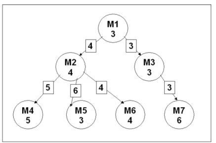
In Figure 1 (taken from Mishra et al. [9]), DCCLoad of modules are calculated.

As an example, for moduleM₂, we have:

m₂= 4 (3.14)

(6)

Figure 1: An example task graph for showing the calculation of DCCLoadfor the allocation {M1, M3, M7}{M2, M6}{M4, M5}.

(DCCLoadi)1≤i≤7 = (-1, -3, 0, 0, -3, 0, 0)

The number of incoming edges that are from different clusters are:

c_in2= 1 (3.15)

The number of outgoing edges that are to different clusters are:

c_out2= 2 (3.16)

The sum of weight of incoming edges that are from different clusters are:

sum_in₂=w₁₃= 4 (3.17) The sum of weight of outgoing edges that are to different clusters are:

sum_out₂=w₂₄+w₂₅= 11 (3.18) ThereforeDCCLoad₂ is given by:

DCCLoad₂= (c_in₂+c_out₂)m₂−sum_in₂−sum_out₂= 12−4−11 =−3 (3.19)

4. The D ynamic CCL oad algorithm

4.1. E valuate -DCCL oad

Evaluate-DCCLoad(T, cluster) 01fori←1to|V|

(7)

02 doc_in[i]←0 03 c_out[i]←0 04 sum_in[i]←0 05 sum_out[i]←0 06fori←1to|V|

07 doload[i].index←i 08 foreach(i, j)∈E

09 do if cluster[i]6=cluster[j]

10 thenf ←1

11 elsef ←0

12 c_in[j]←c_in[j] +f 13 c_out[i]←c_out[i] +f

14 sum_in[j]←sum_in[j] +f wij

15 sum_out[i]←sum_out[i] +f wij

16fori←1to|V|

17 doload[i].value←(c_in[i] +c_out[i])mi−sum_in[i]−sum_out[i]

18returnload

Given a task graphT, the algorithm Evaluate-DCCLoadcalculates theDCC Load for each module in the array load. Using the notation of Mishra et al. [9], for(1≤j≤ |V|), if theDCCLoadof moduleM_j isl_j, and if it is stored inload[i], then we have:

load[i].value=lj (4.1)

and

load[i].index=j (4.2)

In lines 01 to 05, the count (c_in[i]) and the sum of weights of incoming edges from different clusters (sum_in[i]), and the count (c_out[i]) and the sum of weight of outgoing edges to different clusters (sum_out[i]) are initialized to0. In lines 06 to 15, we consider each edge(i, j)∈E, and update the values ofc_out[i],c_in[j], sum_out[i] and sum_in[j] accordingly. Finally, in lines 16 to 17, we store the DCCLoad of module M_i in load[i] for (1 ≤ i ≤ |V|). Line 18 returns the load array.

Lines 01 to 05, and lines 16 to 17 each have complexityO(|V|). Lines 06 to 15 have complexity O(|E|). Line 18 has complexity O(1). Therefore, the algorithm Evaluate-DCCLoadhas complexityO(|V|+|E|).

4.2. E valuate -T ime

Given a task graph T, and a clustering cluster, the algorithm Evaluate-Time taken from Mishra et al. [9] calculates the parallel execution time of the clustering.

It is basically based on the event queue model. There are two type of events:

computation completion event, and communication completion event. Events are denoted as 3-tuples (i, j, t). As an example, a computation completion event of moduleM_i, that completes its computation at timet_i will be denoted as(i, i, t_i),

(8)

and a communication completion event of a communication from Mi to Mj, that is finished at timetij will be denoted as (i, j, tij).

There are a total of(|V|+|E|)events out of which|V|events are computation completion events corresponding to each module, and|E|events are communication completion events corresponding to each edge. Mishra et al. [9] has shown the complexity of the Evaluate-Timealgorithm as O((|V|+|E|)log(|V|+|E|)).

4.3. D ynamic CCL oad Algorithm

DynamicCCLoad(T) 01forj←1 to|V| 02 docluster[j]←1

03load←Evaluate-DCCLoad(T, cluster) 04 Sort-Load(load)

05cmax←2 06forj←1 to|V| 07 doi←1

08 t_min←Evaluate-Time(T, cluster) 09 fork←2toc_max

10 docluster[load[j].index]←k 11 time←Evaluate-Time(T, cluster) 12 if time < t_min

13 thentmin←time

14 i←k

15 cluster[load[j].index]←i

16 load←Evaluate-DCCLoad(T, cluster) 17 load[j].value← −∞

18 Sort-Load(load) 19 if i=cmax

20 thencmax←cmax+ 1 21return(tmin, cluster)

We are using the heuristic of Mishra et al. [9]:

(1) We can keep the computational intensive tasks on separate clusters because they mainly involve computation. Such tasks will heavily load the cluster. If we keep these tasks separated, we can evenly balance the computational load.

(2) We can keep the communication intensive tasks on same cluster because they mainly involve communication. If we keep these tasks on the same cluster, we may reduce the communication delays through edge-zeroing.

The DCCLoad-Clustering algorithm implements the above heuristic using the concept ofDCCLoad. Initially all modules are kept in the same cluster (cluster 1, also called theinitial cluster, lines 01 to 02). Given a task graphT, and an initial allocation of modules cluster, line 03 evaluates the DCCLoad of modules. Line 04 sorts the loadarray in decreasing order. c_max (line 05) will be the number of possible clusters that can result, if one module is removed from theinitial cluster, and put on a different cluster (including theinitial cluster).

(9)

We take the modules out from the initial cluster one-by-one (line 06) in decreasing order ofCCLoad(line 10). At the same time we also calculate the parallel execution time, when it is put on all possible different clusters (lines 09 to 11). t_min is used to record the minimum parallel execution time, andiis used to record the corresponding cluster (lines 12 to 14). Finally we put the module on the cluster that gives the minimum parallel execution time (line 15). In line 16 we also set itsDCCLoad value to−∞to make it invalid so that in future we can not use it.

Line 17 re-evaluates the DCCLoadof modules after the change in allocation and line 18 again sorts them in decreasing order.

It may also happen that the parallel execution time was minimum when the module was put alone on a new cluster. In this case we will have to incrementc_max by 1 (lines 19 to 20). Line 21 finally returns the parallel execution time, and the corresponding clustering.

Lines 01 to 02 have complexityO(|V|). Line 03 has complexity O(|V|+|E|).

Line 04 has complexityO(|V|²)if bubble sort is used [6]. Lines 05 and 21 each have complexity O(1). Lines 08 and 11 have complexity O((|V|+|E|)log(|V|+|E|)).

For each iteration of the for loop in line 06, Evaluate-Time (lines 08 and 11) is called a maximum of |V| times (c_max can have a maximum value of|V|, when all modules are on separate clusters). The complexity of the for loop of lines 06 to 20 is dominated by Evaluate-Time that is called a maximum of |V|² times.

Therefore, theforloop has complexityO(|V|²(|V|+|E|)log(|V|+|E|))that is also the complexity of DynamicCCLoadalgorithm.

5. A simple example

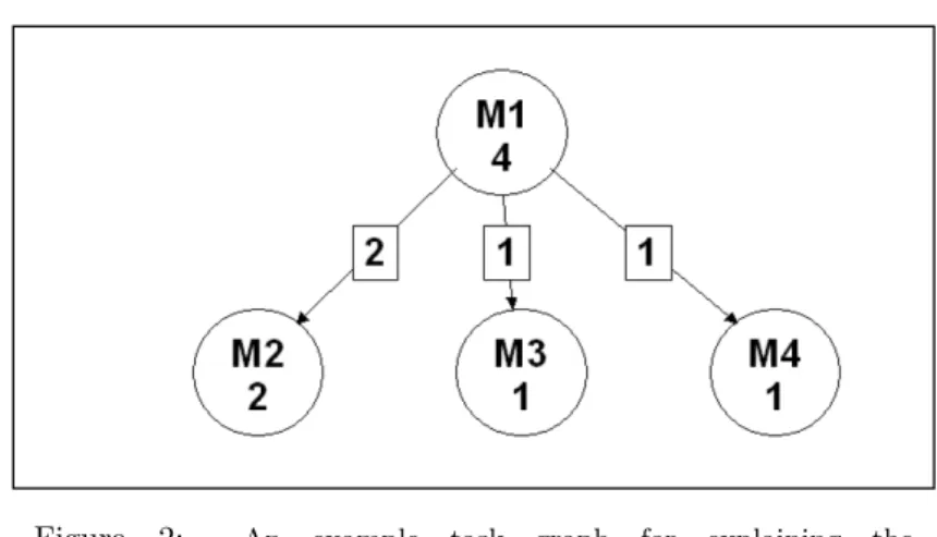
Consider the task graph in Figure 2 (taken from Mishra et al. [9]). Initially all modules will be clustered in theinitial clusteras(cluster[i])_1≤i≤4=(1,1,1,1). Parallel execution time will be8. For the initial allocation we have (DCCLoad_i)_1≤i≤4 = (0,0,0,0). Then the modules are sorted according toDCCLoadin decreasing order as (M₁,M₂,M₃,M₄).

The first module to be taken out isM₁ which forms the clustering (2,1,1, 1).

Parallel execution time for this clustering is9. This is not less than8. Therefore, moduleM₁ is kept back in theinitial cluster as (1,1,1,1). For this allocation we re-calculate DCCLoad. After setting the value of DCCLoad₁ to −∞so that it can not be used in future, we get(DCCLoad_i)_1≤i≤4= (−∞,0,0,0). The modules sorted in decreasing order are: (M2,M3,M4,M1).

We next take out the moduleM₂ to form the clustering (1, 2, 1, 1). Parallel execution time for this clustering is 8. This is also not less than 8. Therefore, moduleM₂ is kept back in theinitial cluster as (1,1,1,1). For this allocation we re-calculate DCCLoad. After setting the value of DCCLoad₂ to −∞so that it can not be used in future, we get (DCCLoad_i)_1≤i≤4 = (−∞,−∞,0,0). Modules sorted in decreasing order are: (M3,M4,M2,M1).

We next take out the moduleM₃ to form the clustering (1, 1, 2, 1). Parallel execution time for this clustering is7. This is less than8. Therefore, moduleM₃

(10)

Figure 2: An example task graph for explaining the DynamicCCLoad algorithm. For the initial allocation we have (DCCLoadi)1≤i≤4 = (0, 0, 0, 0). The DynamicCCLoadalgorithm clusters the modules as (M1,M2)(M3)(M4), giving a parallel exe-

cution time of6.

is kept in a separate cluster as (1, 1, 2, 1). For this allocation we re-calculate DCCLoad. After setting the value of DCCLoad₃ to −∞ so that it can not be used in future, we get (DCCLoad_i)_1≤i≤4= (−∞,−∞,−∞,0). Modules sorted in decreasing order are: (M4, M3,M2,M1).

The last module to be taken out isM4. Now there are two possible clustering:

(1, 1, 2, 2) and (1, 1, 2, 3). Parallel execution time for the clustering (1, 1, 2, 2) is 7. Parallel execution time for the clustering (1, 1, 2,3) is 6. The minimum parallel execution time comes out to be 6 for the clustering (1, 1, 2, 3) that is also less than 7. Therefore, module M₄ is also kept in a separate cluster as (1, 1,2, 3). For this allocation we re-calculateDCCLoad. After setting the value of DCCLoad₄to−∞so that it can not be used in future, we get(DCCLoad_i)_1≤i≤4= (−∞,−∞,−∞,−∞). Modules sorted in decreasing order are: (M₄,M₃,M₂,M₁).

At this point the DynamicCCLoadalgorithm stops.

The final clustering of modules is (M1,M2)(M3)(M4) in which the modulesM1

andM2are clustered together, while the modulesM3andM4are kept on separate clusters. This clustering gives a parallel execution time of 6.

6. Experimental results

The DynamicCCLoadalgorithm is compared with the Sarkar’s edge zeroing algorithm [12]. This algorithm has a complexity ofO(|E|(|V|+|E|)).

Algorithms are tested on benchmark task graphs of Tatjana and Gabriel [3], [2]. We have tested for 120 task graphs having number of nodes: 50,100,200, and 300 respectively. Each task graph has a label astn_i_j.td. Herenis the number

(11)

Figure 3: Parallel execution times for tn_i_j.td.

of nodes. iis a parameter depending on the edge density. Its possible values are:

20, 40, 50, 60, and 80. For each combination of nand i, there are 6 task graphs that are indexed by j. j ranges from1 to 6. Therefore, for each n, there are 30 task graphs.

For the values ofnhaving50,100,200, and300, Figure 3 shows the comparison between the Sarkar’s edge zeroing algorithm and the DynamicCCLoadalgorithm for the parallel execution time. It is evident from the figures that the average improvement of DynamicCCLoadalgorithm over Sarkar’s edge zeroing algorithm ranges from5.81%for100-node task graphs to8.30%for300-node task graphs.

7. Conclusion

We developed the idea ofDCCLoadof a module by including the current allocation of modules. This resulted in a dynamically changing priority of modules. We used a heuristic based on it to develop the DynamicCCLoadalgorithm of complexity O(|V|²(|V|+|E|)log(|V|+|E|)). We also demonstrated its superiority over the Sarkar’s edge zeroing algorithm in terms of parallel execution time. For the future work there are two possibilities: experiment with different dynamic priorities, and experiment with different ways in which we can take the modules out from the initial cluster.

Acknowledgements. The authors are thankful to the anonymous referees for valuable comments and suggestions in revising the manuscript to the present form.

Corresponding author greatly acknowledge the financial assistance received under sponsored research project from the CSIR, New Delhi.

(12)

References

[1] Cormen, T. H., Leiserson, C. E., Rivest, R. L., Stein, C., Introduction to Algorithms, The MIT Press, 2’nd Edition, (2001).

[2] Davidovic, T., Benchmark task graphs available online at: http://www.mi.sanu.

ac.rs/~tanjad/sched_results.htm, (2006).

[3] Davidovic, T., Crainic, T. G., Benchmark-problem instances for static scheduling of task graphs with communication delays on homogeneous multiprocessor systems, Computers and Operations Research, 33(8), (2006) 2155–2177.

[4] Freund, R. F., Siegel, H. J., Heterogeneous processing,IEEE Computer, 26(6), (1993) 13–17.

[5] Horowitz, E., Sahni, S., Rajasekaran, S., Fundamentals of Computer Algo- rithms, W. H. Freeman, (1998).

[6] Langsam, Y., Augenstein, M. J., Tenenbaum, A. M.,Data Structures Using C and C++, Prentice Hall, 2’nd edition, (1996).

[7] Kadamuddi, D., Tsai, J. J. P., Clustering algorithm for parallelizing software systems in multiprocessors environment,IEEE Transations on Software Engineering, 26(4), (2000) 340–361.

[8] Maheswaran, M., Braun, T. D., Siegel, H. J., Heterogeneous distributed computing,J.G. Webster (Ed.), Encyclopedia of Electrical and Electronics Engineering, 8, (1999) 679–690.

[9] Mishra, P. K., Mishra, K. S., Mishra, A., A clustering heuristic for multiprocessor environments using computation and communication loads of modules, International Journal of Computer Science & Information Technology, 2(5), (2010) 170–182.

[10] Mishra, A., Tripathi, A. K., An extension of edge zeroing heuristic for scheduling precedence constrained task graphs on parallel systems using cluster dependent priority scheme,Journal of Information and Computing Science, 6(2), (2011) 83–96.

An extended abstract of this paper appears in the Proceedings of IEEE International Conference on Computer and Communication Technology (ICCCT’10), (2010) 647- 651.

[11] Papadimitriou, C. H., Yannakakis, M., Towards an architecture-independent analysis of parallel algorithms,SIAM Journal on Computing, 19(2), (1990) 322–328.

[12] Sarkar, V.,Partitioning and Scheduling Parallel Programs for Multiprocessors, Re- search Monographs in Parallel and Distributed Computing, MIT Press, (1989).

[13] Siegel, H. J., Dietz, H. G., Antonio, J. K., Software support for heterogeneous computing, A. B. Tucker Jr. (Ed.), The Computer Science and Engineering Handbook, CRC Press, Boca Raton, FL, (1997) 1886–1909.

[14] Yang, T., Gerasoulis, A., A fast static scheduling algorithm for DAGs on an unbounded number of processors,In Proceedings of the 1991 ACM/IEEE Conference on Supercomputing (ICS’91), (1991) 633–642.

[15] Yang, T., Gerasoulis, A., PYRROS: Static task scheduling and code generation for message passing multiprocessors,In Proceedings of the 6’th International Confer- ence on Supercomputing (ICS’92), (1992) 428–437.