Volume XII Number 4, 2020
Accounting for TFP Growth in Global Agriculture - a Common-Factor- Approach-Based TFP Estimation
Lajos Baráth, Imre Fertő
Institute of Economics, Centre for Economic and Regional Studies, Budapest,Hungary
Abstract
There is no consensus about trends in agricultural productivity among agricultural economists. The aim of this paper is to contribute to the investigation of this issue by estimating a Total Factor Productivity (TFP) index for global agriculture and global agricultural regions. One of the biggest challenges with analysing global productivity trends is the lack of price data or cost shares, especially in developing countries.
We apply recently introduced econometric models that permit accounting for technology heterogeneity and the time-series properties of data to estimate cost shares. Aggregate sectoral data from the USDA ERS database are investigated for the period 1990 to 2013. Although we used a different method, our results are in line with earlier findings that used USDA or FAO database. TFP growth has accelerated in world agriculture, largely due to better performance in transition countries. Although TFP growth has accelerated in world agriculture, it has slowed down in industrialized countries. TFP growth in the EU has increased, but at slower rate in recent years. In the Old Member States the growth rate has decreased, whereas in the New Member States it has increased. The results highlight that insufficient spending on productivity-enhancing agricultural R&D in industrialized countries may put future agricultural productivity growth at risk.
Keywords
Total Factor Productivity (TFP), agricultural productivity, heterogeneous technology, time series properties, cross sectional dependence.
Baráth, L. and Fertö, I. (2020) “Accounting for TFP Growth in Global Agriculture - a Common-Factor- Approach-Based TFP Estimation", AGRIS on-line Papers in Economics and Informatics, Vol. 12, No. 4, pp. 3-13. ISSN 1804-1930. DOI 10.7160/aol.2020.120401.
Introduction
Although much work has been done on analysing trends in agricultural productivity, understanding of this issue remains far from complete. Even among agricultural economists that study productivity, there is no consensus about whether the rate of growth in agricultural productivity is slowing (Fuglie and Wang, 2012). Recently, Alston, Babcock, and Pardey (2010) examined a number of studies about trends in agricultural productivity in various regions of the world. Their conclusion was that "agricultural productivity has slowed, especially in the world’s richest countries.” But they also recognized that the evidence was mixed, and, given the importance of the issue, that it needed further investigation (Fuglie and Wang, 2012).
The goal of this paper is to contribute to the investigation of this issue. We use recently introduced methodological developments to provide insight into the questions: (i) whether global agricultural TFP growth has slowed down
in recent decades, and (ii) whether the slowdown in productivity is more significant in industrialized countries. Additionally, we investigate the evolution of TFP growth in the European Union and examine the differences in TFP growth between Old and New Member States.
TFP is usually defined as the ratio of aggregate output to aggregate input. It is therefore necessary to account for the sum of changes of outputs and inputs used in production. We apply the ‘growth accounting’ method.
The growth accounting method measures aggregate input growth as the weighted sum of the growth rates of the quantities of the individual factors of production, wherein the weights are the cost shares. In the case of outputs, revenue shares are used. However, for most countries in the world there is a lack of representative data about input prices and therefore cost shares. This is especially true for developing countries, where the most important inputs are farm-supplied, like land and labour,
but where wage labour and land rental markets are thin, making it difficult to assess the share of these inputs in total cost (Alston, Babcock and Pardey, 2010; Fuglie, 2012).
To deal with this challenge, most examinations of global agricultural TFP have relied on distance function measures (like the Malmquist index) to compare productivity among groups of countries.
Distance functions are derived from input- output relationships based on quantity data only:
for example, Ludena (2010) and Coelli and Rao (2005) applied this method. However, this methodology is sensitive to the set of countries that is included for comparison and the number of variables in the model, and the dimensionality issue (Alston, Babcock and Pardey 2010; Fuglie, 2012; Lusigi and Thirtle, 1997).
Another way of dealing with the lack of input prices was proposed by Avila and Evenson who used input cost shares estimated from agricultural censuses in Brazil and India to impute cost shares for other developing countries. In contrast to many DEA models which found that agricultural TFP growth was negative, the former authors reported positive and accelerating TFP growth for developing countries (Fuglie, 2015; Dias Avila and Evenson, 2010).
Alternatively, econometric estimates of a production function can be used instead of price or cost data. One of the disadvantages of this approach is that it involves strong technical and economic assumptions, like profit maximization and the imposition of a functional form. However, Fuglie argues that imposing more structure could be an advantage when dealing with data with a high degree of measurement error, as it can help to produce more plausible results (Fuglie, 2012; Nin-Pratt et al., 2015). One of the central focal points of studies that used econometric estimation of empirical cross-country production function over the past two decades has been the endogeneity of inputs and, closely related, potential reverse causality in the estimation equation. In the literature, identification in the face of these difficulties is typically achieved through instrumentation (Eberhardt and Teal, 2017). However, if technology is heterogeneous across countries then none of the standard instrumentation strategies applied in the cross-country empirical literature (such as instrumentation using z variables or lags) are valid, since the empirical specifications in these cases assume technology homogeneity (Eberhardt, 2009). In addition, standard instrumentation strategies also assume stationary variable series,
as well as cross-sectional independence, and this identification strategy is invalid if any of these assumptions are violated (Eberhardt and Teal, 2013a).
We use advances from non-stationary econometrics and apply a common factor framework to model production. This approach is able to account for heterogeneity in technology, the non-stationary, cross-section dependence of data, and endogeneity.
We follow Eberhardt and Teal (2013b) and compare different heterogeneous models with different assumptions concerning technology heterogeneity and the effect of common factors. We base our decision concerning the preferred model on residual diagnostic tests, and we check for non-stationarity and cross-sectional independence of the residuals.
Although the models thus applied can account for endogeneity, we cannot rule out reverse causality. In order to address this issue, we follow Eberhardt-Teal and simply also estimate the Fully Modified Ordinary Least Square (FMOLS) version of the preferred model and compare estimates between the OLS and FMOLS versions of the models (Eberhardt and Teal 2017). Since the FMOLS methodology is robust to reverse causality, this supplies the assurance that if the coefficients are similar in the two versions, then our estimates represent production function coefficients and our model is not misspecified (e.g., not investment or labour demand equations).
In the second step of our analysis we use the parameter estimates of the preferred model to construct the TFP index and answer our empirical questions. We use the USDA-ERS agricultural database, which has a sufficient number of cross- sectional and time-series observations to model production through applying a common factor framework. Moreover, to the best of our knowledge this database has not yet been examined using these types of models.
Materials and methods
We adopt common factor representation for a production function which allows for heterogeneity in technology, as well as for common shocks to production and/or technology spill overs between countries (‘cross-sectional dependence’) The common factor model framework is arguably ideally suited to the analysis of cross-country productivity (Bai, 2009; Chudik, Pesaran and Tosetti, 2011) but has thus far not been applied very widely
(Cavalcanti, Mohaddes and Raissi, 2011; Eberhardt and Teal, 2013a; Eberhardt and Teal, 2013b).
We follow Eberhardt and Teal (2013a) and we modell production in country i at time t, for i = 1, . . . , N, t = 1, . . . , T and m = 1, . . . , k as follows:
(1)
(2)
and (3)
This technique has been shown to be extremely powerful and can provide consistent estimates of βi' or its cross-country average, even if factors are non-stationary, if there are structural breaks in the factors, or whether there is cointegration or non-cointegration between the model variables (Eberhardt and Teal, 2017).
We follow the existing literature and include proxies for labour, agricultural capital, livestock, fertilizer, and land under cultivation as the m observed inputs xit in the model for observed output yit (all variables in logarithms). As Equation 1 shows, uit is represented by a combination of country- specific fixed effects αi and a set of common factors ft with factor loadings that can differ across countries (λi). Equation (3) specifies the evolution of the common factors and includes the potential for non-stationary factors (ϱ = 1, k = 1) and thus non-stationary inputs and outputs (Eberhardt and Teal, 2013a).
Some of the unobserved common factors driving the variation in yit in Equation (1) also drive the regressors in (2). This setup induces endogeneity in that the regressors are correlated with the unobservables in the production function equation (uit), making it difficult to identify βi separately from λi and ρi (Kapetanios, Pesaran and Yamagata, 2011; Eberhardt and Teal, 2017).
In the literature, identification in the face of these difficulties is typically argued to be achieved through instrumentation. However, if any of the assumptions of homogeneous technology, stationary variable series, or cross-sectional independence are violated, the identification strategy through instrumentation may be deemed invalid (Eberhardt and Teal, 2017). In the common factor framework, the resulting endogeneity problem can be tackled by accounting for the presence of the unobservables in the empirical specification (Eberhardt and Teal, 2017; Pesaran and Smith, 1995). In addition, by using diagnostic tests it
is possible to check whether the endogeneity concern has been addressed: "By investigating whether residual series are cross-sectionally correlated we can highlight to what extent we have been able to deal with the dependence caused by the unobservable factors and thus indirectly whether we have addressed the endogeneity concern: if residuals are white noise we know that empirical results do not suffer from endogeneity bias specification” (Eberhardt and Vollrath, 2018).
In the empirical section of this paper we employ and compare different heterogeneous models:
(1) Pesaran and Smith (1995) mean group (MG), (2) the heterogeneous version of the CCE estimators (CCEMG), and (3) the Augmented Mean Group Estimator (AMG) (Eberhardt-Teal, 2013a).
All of the employed models make different assumptions regarding βi, λi, αi, as well as regarding the persistence of the underlying common factors in equations (1)-(3). A detailed description of these models can be found in many papers, thus for reasons of brevity we direct interested readers to Eberhardt (2009); Eberhardt and Teal (2013);
Eberhadt-Teal (2017); Pesaran (2006), and Pesaran and Smith (1995).
If the aim were only to estimate some form of average agricultural technology, the mean of the estimated βi values across all countries could be used. Alternatively, we could look at the average value of βi-s across sub-groups of countries.
Averaging across alternative groups enables us to identify the central tendencies in technology parameters. However, it is important to note that country-specific parameter coefficients should not be viewed in isolation (Pedroni, 2007) because they frequently yield economically implausible magnitudes (Boyd and Smith, 2002; Eberhardt and Teal, 2013a). In other words, each estimate is a noisy signal of the true parameter value, and averaging across groups of countries boosts this signal and reduces noise (Eberhardt and Vollrath 2018). Therefore, we use for further empirical analysis only the averages of the estimated βi values across all countries and across sub-groups of countries.
In the second step of our analysis we used the averages of the βi values of the preferred model to calculate the TFP index, similarly to Fuglie (2010; 2015):
(4) where Ri is the revenue share of the ith output
and Sj is the cost share of the jth input.
TFP growth is calculated as the difference in aggregate output and the growth in aggregate input. For the empirical examination we used the gross agricultural output from USDA database and aggregated the inputs using the elasticities of the preferred model that was chosen in the first step of our analysis.
One limitation of this method of calculation is that the cost shares are held constant. However, Fuglie (2010) reports with reference to the applied database that there has been movement among the major input categories, but these changes have occurred gradually (over decades). Thus, the likelihood of major biases in productivity measurement over a decade or two is not large. As our aim is to calculate productivity over two decades (1990-2013), the bias in our case is certainly not large.
We employ aggregate sectoral data for agriculture from the USDA ERS database for the period 1990 to 20131. The applied sample represents an unbalanced panel of 173 countries with 24 time-series observations. A detailed description of the variables can be found on the homepage for the USDA ERS database2. For output variable (y) we use gross agricultural output measured in international 2005 $. We use five input variables: land, fertilizer, machinery, livestock, and labour.
Land (X1) represents total agricultural land in hectares of ‘rainfed cropland equivalents’3.
1 Database downloaded in March 2017.
2 https://www.ers.usda.gov/data-products/international-agricultural- productivity/
3 This is the sum of rainfed cropland (weight equals 1.00), irrigated cropland (weight varies from 1.00 to 3.00 depending on region) and permanent pasture (weight varies from 0.02 to 0.09 depending on region). https://www.ers.usda.gov/data-products/international- agricultural-productivity/.
Fertilizer (X2) represents metric tonnes of N, P2O5, and K2O fertilizer consumption. The livestock variable (X3) is the total livestock capital on farms in ‘cattle equivalents.’ Machinery (X4) is the total stock of farm machinery in '40-CV tractor equivalents'. Labour (X5) represents the number of economically active adults engaged in agriculture.
Results and discussion
Parameter estimates of the applied models Table 1 displays the results of estimated models.
For all models we report residual diagnostic tests, namely the Pesaran (2007) panel unit root test and the Pesaran (2004) CD test. We use residual diagnostics to choose the preferred empirical models. Further details about the importance of residual diagnostics in empirical modelling can be found in Eberhardt and Teal (2011) and Banerjee and Carrion-i-Silvestre (2015).
All heterogeneous models yield statistically significant technology coefficients, suggesting that the average technology is different among countries.
The estimates of CCEMG and AMG models are similar, whereas the estimated coefficients of the MG model are different. One explanation for this is revealed in simulation studies:
for non-stationary and cross-sectionally dependent data, the MG estimates are severely affected by failure to account for cross-sectional dependence (Coakley, Fuertes, and Smith 2006; Eberhardt and Bond, 2009).
All models yield stationary residuals; however, only the AMG model yields both cross-sectionally independent and stationary residuals. This suggests that the AMG model is a better fit for the database.
Although the AMG model is able to account for technology heterogeneity, cross-sectional
1_MG 2_CCEMG 3_AMG
Coef. P>|t| Coef. P>|t| Coef. P>|t|
l_land 0.27 0.00 0.19 0.00 0.22 0.00
l_mat 0.02 0.01 0.02 0.01 0.02 0.00
l_cap 0.12 0.04 0.15 0.00 0.10 0.06
l_liv 0.26 0.00 0.18 0.00 0.19 0.00
Stationarity I(0) I(0) I(0)
CD 3.4 (0.001) 2.52(0.012) 1.32(0.187)
Note: I(1) stands for stationary residual; I(0) represents non-stationary residual; CD shows the Pesaran (2004) CD statistic, and in brackets the p-value; H0: cross-sectionally independent residual
Source: Authors’ calculations
Table 1: Parameter estimates and residual diagnostics of heterogeneous models.
dependence non-stationarity and endogeneity, we cannot rule out reverse causality. To address this issue, we estimated the (FMOLS) version of this model and compared the resulting estimates with the OLS-based version (Table 2). FMOLS methodology is robust to reverse causality:
if the coefficients are similar in the two versions then we can rule out the issue of reverse causality and can be sure that our estimates represent production function coefficients. Results of the comparison of OLS- and FMOLS- based estimates are very similar, thus we used the estimates of the AMG model for further empirical analysis.
Variable Coefficient t-Statistic
l_land 0.20 30.96
l_mat 0.02 8.58
l_cap 0.12 13.86
l_liv 0.19 36.20
Note: Model was estimated in RATS Source: Authors’ calculations
Table 2: AMG Model using FMOLS.
TFP growth in industrialized, developing, and transition countries
As Fuglie (2010) reported, recent assessments of the global agricultural economy have expressed concern about a significant slow-down in productivity growth. Yet, evidence from major developing countries suggests that productivity
growth has accelerated in these regions. This contrasts with the findings of earlier studies of global productivity growth, which found agricultural land and labour productivity rising faster in developed than in developing countries (Hayami and Ruttan, 1985; Craig, Pardey and Roseboom, 1997). Another confounding factor is the uneven performance of agriculture in transition countries. Thus, national and regional evidence is mixed concerning recent trends in agricultural productivity.
The results of more recent papers are also contradictory. Alston and Pardey (2014) find that the global rate of agricultural productivity growth is declining, whereas Fuglie (2015) reports that there has been significant acceleration in global agricultural productivity growth since the 1990s.
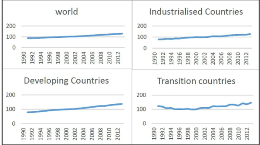
Our results are shown in Figure 1. and Table 3.
Figure 1 shows the evolution of TFP growth (2000=100%) over the period under analysis, and Table 4 shows the difference in the average annual growth rates for two periods: 1991-2000, and 2011-2012.
Figure 1 shows that TFP growth has increased in global agriculture (world), industrialized (IND), developing (DEV) and transition countries (TRA) compared to 2000 (Figure 1). However, there are remarkable differences in the average annual growth rates in the analysed periods (Table 3).
Examination of average annual TFP growth rates prior and post-2000 shows that TFP growth has
Periods World IND TRA DEV
1991-2000 1.74% 2.58% -2.21% 2.77%
2001-2013 2.10% 2.07% 2.36% 2.66%
Source: Authors’ estimation
Table 3: Average annual growth rate of TFP in global agriculture.
Source: Authors’ estimation
Figure 1: Evolution of TFP growth in global agriculture (2000=100%).
accelerated in world agriculture. It slowed down in industrialized countries, remained nearly at the high-level earlier characteristic of developing countries, and accelerated in transition countries (Table 3).
Although we used different methods to estimate cost shares, our estimates are similar to the USDA estimates (Appendix 1). This suggests that the method we used gives plausible results and is adequate for estimating TFP growth, especially in countries where prices are not available.
These estimates suggest, similarly to earlier findings in the literature, that the acceleration of global TFP growth in recent decades has largely been due to better performance in developing countries and transition economies.
According to Fuglie (2010; 2015), two large developing countries are leading in terms of growth:
China, and Brazil, while very recently agricultural TFP growth in India has also accelerated.
In industrialized countries our estimates also confirm earlier findings (Fuglie, 2010; 2015):
resources from agriculture are being withdrawn from agriculture at an increasing rate. The average annual growth rate of inputs according to our calculations was -1.2 % from 1991-2000 and was -1.43% from 2001-2013. This calls attention to the same fact that Alston and Pardey (2014) highlight in their paper: insufficient spending on productivity-enhancing agricultural R&D in industrialized countries may put future agricultural productivity growth at risk.
In transition countries at the beginning of 1990s TFP growth slowed down significantly, then in the middle of 1990s started to accelerate.
At the beginning of the 2000s the growth rate increased considerably (Figure 1). These results are in line with earlier findings from the literature.
Swinnen and Vranken (2010) conducted a detailed examination that involved applying different methods to investigate the changes in productivity in transition countries from 1989-2005. The authors revealed that there have been dramatic changes in productivity over this period in transition countries. In general, one observes a J-shaped (or U-shaped) effect: an initial decline in productivity, and a later recovery. Virtually all countries witnessed an initial decline in productivity, followed by an increase in productivity in the 2000s, and in several transition countries the growth in productivity since 2000 has been quite spectacular (Swinnen and Vranken, 2010). Our graph shows a similar
pattern and reveals that in the years following the last year of their examination (2005) productivity also continued to follow this pattern (Figure 1).
TFP growth in the EU
The increase in agricultural productivity has attracted renewed interest in the EU for a number of reasons. First, the European Commission has launched an ambitious program to promote a more resource-efficient Europe by 2020.
As a consequence, the agricultural sector is challenged to do more with less. Second, TFP is one of the three impact indicators used in determining the success of the general CAP objective of promoting viable food production. Impact indicators measure the outcome of an intervention beyond its immediate effects. Third, TFP is also used to evaluate the European Innovation Partnership for Agricultural Productivity and Sustainability (EIP-Agri3) (EC, 2016).
The European Commission in 2016 reported that both in the EU-15 and the EU-N13 TFP growth has increased over the period 1995-2005, and it is remarkable that the high growth rate of the EU-N13 is offset by the lower growth rate in the EU- 15; the EU-N13 growth rates are relatively high (over 1.6%/year). In the associated paper the Fisher index was used to estimate TFP, and the Economic Accounts for Agriculture (EAA) database.
In a recent paper, Baráth and Fertő (2017) using the DEA Method constructed a Lowe TFP index based on EAA data and found that TFP slightly decreased in the EU over the period 2004-2013;
however, there are significant differences between the OMS and NMS and across Member States.
Our present findings about TFP development in the EU and the OMS and NMS are shown in Figure 2 and Table 4. Figure 2 shows the evolution of TFP growth (2000=100%) while Table 4 shows the average annual growth rates in the 1990s (1991-2000) and 2000s (2000-2013).
Our findings show that TFP growth in the EU has increased over time, although at a slightly slower rate in recent years than in the past. While the growth rate was around 1.2% per year between 1991 and 2000, it had slowed down to around 1.1%
between 2001 and 2013.
The differences between the OMS and NMS are remarkable. In the OMS, the growth rate was around 1.7% per year between 1991 and 2000, whereas during this time in the NMS it was only 0.10 %.
In the OMS the growth rate slowed down to around 1%; in contrast, in the NMS it was around 1.3 %.
Periods EU OMS NMS
1991-2000 1.22% 1.66% 0.10%
2001-2013 1.11% 1.04% 1.31%
Source: Authors’ estimation
Table 4: TFP average annual growth in EU, Oms and NMS.
Source: Authors’ estimation
Figure 2: Evolution of TFP growth in the EU (2000=100%).
Direct comparison of these results with those of other studies is difficult because different studies use different groupings and time periods. The EC reports results for the EU-28, EU-15 and EU-N13, whereas the USDA reports results for Europe Northwest, Europe Southern, Europe Transition and Europe Baltic. In the USDA database, 29 European countries can be found, among which 25 EU member states, 14 OMS and 11 NMS.
Therefore, we compared our results to the most similar groups (Appendix 2). The comparison shows that in the case of EU estimates our results are similar to those of the USDA, while the EC estimates are much lower. As the EC used the EAAE database, which has more specific variables, the result of our comparison suggests and confirms our earlier finding that FAO database-based analyses likely overestimate productivity growth in the EU (Baráth-Fertő, 2017).
Conclusions
Recent assessments of the global agricultural economy have expressed concern about a significant slowdown in productivity growth (Fuglie, 2010).
The first aim of this paper was to examine whether global agricultural productivity has indeed slowed down using recently introduced models which allow us to consider the technological heterogeneity and time-series properties of the data. Our second
aim was to examine the differences in TFP growth in global agricultural regions (namely, in industrialized, transition and developing countries), as well as in the EU and its OMS and NMS.
We used diagnostic tests to select the preferred model for further empirical analysis. The results of these showed that the recently introduced AMG model better fits these data.
Our empirical results showed that TFP growth has accelerated in world agriculture over the last two decades. The estimates suggest and confirm earlier findings in the literature that the acceleration of global TFP growth in recent decades has been due to better performance in developing countries and the transition economies (Fuglie, 2010; 2015).
Although we used a different method to the USDA to obtain factor shares, our results are closely in line with their estimates. This suggests that the applied methods give plausible results and can be used to evaluate TFP for global regions and can help to estimate TFP in regions where prices or cost shares are not available.
Our findings show that TFP growth in the EU has increased over time, although at a slightly slower rate in recent years than in the past decade. Differences between the OMS and NMS are remarkable.
In the OMS the growth rate has significantly
decreased, whereas in the NMS there was a remarkable increase in TFP growth in the last decade. These results are also in line with USDA estimates, but are at odds with EAA-based estimates.
This confirms our earlier finding that FAO-data- based analyses likely overestimate productivity growth in the EU (Baráth-Fertő, 2017).
Although TFP growth has accelerated in world agriculture, it has slowed down in industrialized countries. The most important factor determining productivity growth in the long term is innovation, which is driven by research investment.
The conceptualization of this process according to Fuglie –Heisey (2007) is as follows: expenditures on agricultural research generate new knowledge that eventually leads to improved technology that is adopted by farmers and technology adoption increases average productivity.
Most studies find a significant positive effect for the productivity of investment in innovative
technologies (EC, 2016). Therefore, for stopping or reversing the slowdown in TFP growth in industrialized countries, sufficient spending on agricultural R&D is essential. Additionally, political instruments can increase or decrease TFP growth. However, the link between single political instruments and productivity is not clear;
the results of related studies are mixed, especially in the case of agricultural subsidies. Further research which increases understanding of the channels through which agricultural policy instruments affect productivity is also important for improving productivity growth.
Acknowledgments
Lajos Baráth gratefully acknowledges support from National Research Development and Innovation Office (Hungary); project no. K120326.
Corresponding authors Lajos Baráth
Institute of Economics, Centre for Economic and Regional Studies, Tóth Kálmán u. 4, 1097 Budapest, Hungary
Phone: +36 30 473 03 12, E-mail: barath.lajos@krtk.mta.hu ORCID: https://orcid.org/0000-0002-7137-2376
References
[1] Alston, J. M., Babcock, B. A. and Pardey, P. G. (2010) "The Shifting Patterns of Agricultural Production and Productivity Worldwide", The Midwest Agribusiness Trade Research and Information Center, Iowa State UNiversity, Ames, Iowa. ISBN 978-0-9624121-8-9.
[2] Alston, J. M., and Pardey, P. G. (2014) “Agriculture in the Global Economy”, Journal of Economic Perspectives, Vol. 28, Bo. 1, pp. 121-146. ISSN 08953309. DOI 10.1257/jep.28.1.121.
[3] Bai, J. (2009) “Panel Data Models with Interactive Fixed Effects”, Econometrica, Vol. 77, No. 4, pp.
1229-1279. E-ISSN 1468-0262. DOI 10.3982/ECTA6135.
[4] Baltagi, B. H., Bresson, G. and Pirotte, A. (2007) “Panel Unit Root Tests and Spatial Dependence”, Journal of Applied Econometrics, Vol. 22, No. 2, pp. 339-360. E-ISSN 1099-1255.
DOI 10.1002/jae.950.
[5] Banerjee, A. and Carrion-i-Silvestre, J. L. (2015) “Cointegration in Panel Data with Structural Breaks and Cross-Section Dependence”, Journal of Applied Econometrics, Vol. 30, No. 1, pp. 1-23.
E-ISSN 1099-1255. DOI 10.1002/jae.2348.
[6] Baráth, L. and Fertő, I. (2017) “Productivity and Convergence in European Agriculture”, Journal of Agricultural Economics, Vol. 69, No. 1, pp. 228-248. E-ISSN 1477-9552.
DOI 10.1111/1477-9552.12157.
[7] Cavalcanti, V. de V. , T., Mohaddes, K. and Raissi, M. (2011) “Growth, Development and Natural Resources: New Evidence Using a Heterogeneous Panel Analysis”, Quarterly Review of Economics and Finance, Vol. 51, No. 4, pp. 305-318. ISSN 1062-9769. DOI 10.1016/j.qref.2011.07.007.
[8] Chudik, A., Pesaran, M. H. and Tosetti, E. (2011) “Weak and Strong Cross-Section Dependence and Estimation of Large Panels”, Econometrics Journal, Vol. 14, No. 1. E-ISSN 1368-423X, ISSN 1368-4221. DOI 10.1111/j.1368-423X.2010.00330.x.
[9] Coakley, J., Fuertes, A.-M. and Smith, R. (2006) “Unobserved Heterogeneity in Panel Time Series Models”, Computational Statistics & Data Analysis, Vol. 0, No. 9, pp. 2361-2380. ISSN 0167-9473.
DOI 10.1016/j.csda.2004.12.015.
[10] Coelli, T. J. and Rao, D. S. P. (2005) “Total Factor Productivity Growth in Agriculture:
A Malmquist Index Analysis of 93 Countries, 1980-2000”, Agricultural Economics, Vol. 32, No. 1, pp. 115-134. E-ISSN. DOI 10.1111/j.0169-5150.2004.00018.x.
[11] Craig, B. J., Pardey, P. G. and Roseboom, J. (1997) “International Productivity Patterns: Accounting for Input Quality, Infrastructure, and Research”, American Journal of Agricultural Economics, Vol. 79, No. 4. pp. 1064-1076. E-ISSN 1467-8276. DOI 10.2307/1244264.
[12] Dias, A., Flavio, A. and Evenson, R. E. (2010) “Chapter 72 Total Factor Productivity Growth in Agriculture. The Role of Technological Capital”, Handbook of Agricultural Economics, Vol. 4, pp. 3769-3822. ISSN 1574-0072. DOI 10.1016/S1574-0072(09)04072-9.
[13] Eberhardt, M. and Bond, S. (2009) “Cross-Section Dependence in non-stationary Panel Models:
A Novel Estimator”, Social Research, MPRA Paper,University Library of Munich, Germany.
[14] Eberhardt, M. and Teal, F. (2011) “Econometrics for Grumblers: A New Look at the Literature on Cross-Country Growth Empirics”, Journal of Economic Surveys, Vol. 25, No. 1, pp. 109-155.
E-ISSN 1467-6419. DOI 10.1111/j.1467-6419.2010.00624.x.
[15] Eberhardt, M. and Teal, F. (2013a) “No Mangoes in the Tundra: Spatial Heterogeneity in Agricultural Productivity Analysis”, Oxford Bulletin of Economics and Statistics, Vol. 75, No. 6, pp. 914-939.
E-ISSN 1468-0084. DOI 10.1111/j.1468-0084.2012.00720.x.
[16] Eberhardt, M. and Teal, F (2013b) “Structural Change and Cross-Country Growth Empirics”, World Bank Economic Review, Vol. 27, No. 2, pp. 229–271. E-ISSN 1564-698X, ISSN 0258-6770.
DOI 10.1093/wber/lhs020.
[17] Eberhardt, M. and Vollrath, D. (2018) “The Effect of Agricultural Technology on the Speed of Development”, World Development, Vol. 109, pp. 483-496. ISSN 0305-750X.
DOI 10.1016/j.worlddev.2016.03.017.
[18] Fuglie, K. and Wang, S. L. (2012) “Productivity Growth in Global Agriculture”, Population and Development Review, Vol. 39, No. 2, pp. 361-365. ISSN 00987921.
[19] Fuglie, K. (2015) “Accounting for Growth in Global Agriculture”, Bio-Based and Applied Economics., Vol. 4, No. 3, pp. 201-234. E-ISSN 2280-6172, ISSN 2280-6180.
DOI 10.13128/BAE-17151.
[20] Fuglie, K. (2012) "Productivity Growth and Technology Capital in the Global Agricultural Economy", In "Productivity Growth in Agriculture: An International Perspective", CABI e-Book, Chater No. 16, 333 p. ISBN 9781845939212. DOI 10.1079/9781845939212.0335.
[21] Fuglie, K. and Heisey, P. W . (2007) "Economic Returns to Public Agricultural Research", Economic Brief, Nr. 10, USDA Economic Research Service.
[22] Jerzmanowski, M. (2007) “Total Factor Productivity Differences: Appropriate Technology vs. Efficiency”, European Economic Review, Vol 51, No. 8, pp. 2080-2110. ISSN 0014-2921.
DOI 10.1016/j.euroecorev.2006.12.005.
[23] Kapetanios, G., Pesaran, M. H. and Yamagata, T. (2011) “Panels with Non-Stationary Multifactor Error Structures”, Journal of Econometrics, Vol. 160, No. 2, pp. 326-348. ISSN 0304-4076.
DOI 10.1016/j.jeconom.2010.10.001.
[24] Ludena, C. E. (2010) “Agricultural Productivity Growth, Efficiency Change and Technical Progress in Latin America and the Caribbean”, Inter-American Development Bank.
DOI 10.2139/ssrn.1817296.
[25] Lusigi, A., and Thirtle, C. (1997) “Total Factor Productivity and the Effects of R&d in African Agriculture”, Journal of International Development, Vol. 9, No. 4, pp. 529-538.
E-ISSN 1099-1328. DOI 10.1002/(SICI)1099-1328(199706)9:4<529::AID-JID462>3.0.CO;2-U.
[26] Maddala, G. S., and Wu, S. (1999) “A Comparative Study of Unit Root Tests with Panel Data and a New Simple Test”, Oxford Bulletin of Economics and Statistics, Vol. 61, No. S1, pp. 631-652.
E-ISSN 1468-0084. DOI 10.1111/1468-0084.0610s1631.
[27] Mundlak, Y., Butzer, R. and Larson, D. F. (2012) “Heterogeneous Technology and Panel Data:
The Case of the Agricultural Production Function”, Journal of Development Economics, Vol. 99, No. 1, pp. 139-149. ISSN 0304-3878. DOI 10.1016/j.jdeveco.2011.11.003.
[28] Nin-Pratt, A., Falconi, C. Ludena, C. L. and Martel, P. (2015) “Productivity and the Performance of Agriculture in Latin America and the Caribbean”, Inter-American Development Bank.
[29] Pedroni, P. (2007) “Social Capital, Barriers to Production and Capital Shares: Implications for the Importance of Parameter Heterogeneity from a non-stationary Panel Approach”, Journal of Applied Econometrics, Vol. 22, No. 2, pp. 429-451. E-ISSN 1099-1255. DOI 10.1002/jae.948.
[30] Pesaran, M. H. (20077) “A Simple Panel Unit Root Test in the Presence of Cross-Section Dependence”, Journal of Applied Econometrics, Vol. 22, No. 2, pp. 265-312. E-ISSN 1099-1255.
DOI 10.1002/jae.951.
[31] Pesaran, M. H. and Smith, R. (1995) “Estimating Long-Run Relationships from Dynamic Heterogeneous Panels”, Journal of Econometrics, Vol. 68, No. 1, pp. 79-113. ISSN 0304-4076.
DOI 10.1016/0304-4076(94)01644-F.
[32] Pesaran, M. H., Smith, L. V. and Yamagata, T. (2013) “Panel Unit Root Tests in the Presence of a Multifactor Error Structure”, Journal of Econometrics, Vol. 175, No. 2, pp. 94-115.
ISSN 0304-4076. DOI 10.1016/j.jeconom.2013.02.001.
[33] Pesaran, M. H. (2004) “General Diagnostic Tests for Cross Section Dependence in Panels General Diagnostic Tests for Cross Section Dependence in Panels”, Cambridge Working Papers in Economics 0435, Faculty of Economics, University of Cambridge.
[34] Swinnen, J. and Vranken, L. (2010) “Reforms and Agricultural Productivity in Central and Eastern Europe and the Former Soviet Republics: 1989-2005”, Journal of Productivity Analysis, Vol. 33, pp. 241–258. E-ISSN 1573-0441, ISSN 0895-562X. DOI 10.1007/s11123-009-0162-6.
Appendix
World IND TRA DEV
Own estimates
1991-2000 0.017372 0.025805 -0.00993 0.027712 2001-2013 0.020957 0.02073 0.018062 0.026607
USDA estimates
1991-2000 0.015999 0.020156 -0.00182 0.022024 2001-2013 0.017261 0.020249 0.014529 0.019734 Source: own processing
Appendix 1: Comparison of own estimates with USDA estimates.
Notes:
As similar groupings were not available, we compared the estimates of EC, 2016 to the most similar groups as follows:
1: calculated for all Old Member States available in the USDA database 2: calculated as average of Europe Northwest and Europe Southern
3: calculated for all New Member States (countries that joined the EU after May 2004) available in the USDA database
4: calculated as average of Europe Transition and Europe Baltic 5: calculated for all EU Member States available in the USDA database
6: calculated as average of Europe Northwest, Europe Southern, Europe transition and Europe Baltic
Source: own processing
Appendix 1: Comparison of own estimates with USDA estimates.
1995-2005 2005-2015
EU-15
EC 1.3
EU-15
EC 0.60%
own 1.5 own1 1.31%
USDA 1.48 USDA2 2%
EU-N13
EC 1.60%
own3 2.12%
USDA4 2.11%
EU-28
EC 0.80%
own5 1.45%
USDA6 2.05