TMCrys:predictpropensityofsuccessfortransmembraneproteincrystallization Structuralbioinformatics

(1)

Structural bioinformatics

TMCrys: predict propensity of success for transmembrane protein crystallization

Julia K. Varga

¹

and Ga´bor E. Tusna´dy

^1,

*

1‘Momentum’ Membrane Protein Bioinformatics Research Group, Institute of Enzymology, Research Center of Natural Sciences, Hungarian Academy of Sciences, H-1117 Budapest, Hungary

*To whom correspondence should be addressed.

Associate Editor: Alfonso Valencia

Received on October 13, 2017; revised on March 10, 2018; editorial decision on April 23, 2018; accepted on April 25, 2018

Abstract

Motivation:

Transmembrane proteins (TMPs) are crucial in the life of the cells. As they have special properties, their structure is hard to determine––the PDB database consists of 2% TMPs, despite the fact that they are predicted to make up to 25% of the human proteome. Crystallization predic- tion methods were developed to aid the target selection for structure determination, however, there is a need for a TMP specific service.

Results:

Here, we present TMCrys, a crystallization prediction method that surpasses existing prediction methods in performance thanks to its specialization for TMPs. We expect TMCrys to improve target selection of TMPs.

Availability and implementation:

https://github.com/brgenzim/tmcrys

Contact:

tusnady.gabor@ttk.mta.hu

Supplementary information:Supplementary data

are available at

Bioinformatics

online.

1 Introduction

Transmembrane proteins (TMPs) play vital roles in numerous cell functions being enzymes, receptors or channels, connecting the inner and outer environment of the cells. They may also anchor proteins to the membrane of the cell and play roles in cell–cell recognition and form intercellular joining. About a quarter of the human proteome consists of TMPs (Dobsonet al., 2015b) and around 50% of the marketed drugs interacts with these proteins (Hopkins and Groom, 2002). TMPs have very special physical-chemical properties as they span the hydrophobic cell and organelle membranes, making the determination of their structures extremely difficult. In a recent work, it was found that among the about 3000 human polytopic TMPs only around 60 ones have an experimentally determined structure that covers all of their membrane regions (Varga et al., 2017).

The process of TMP structure determination consists of several steps (Kobeet al., 2008). First, an appropriately designed DNA sequence (Mirzadehet al., 2016) has to be cloned to a suitable expression system and overexpressed in sufficient quantity (Lundstrom, 2006). TMPs tend to be challenging with regards to their expression in larger quantities as they can be toxic to a cell (Gubelliniet al., 2011).

In prokaryotic systems, some post-translational modifications, like gly- cosylation, do not occur and that may prevent the production of the functional protein with the proper structure (Andre´ll and Tate, 2013).

After these problems are overcome, the membrane fraction is separated and the TMPs are solubilized with the appropriate detergents or detergent mixtures. The selection of the proper detergent is a subject to trial- and-error experiments and is often done by high-throughput screenings with a set of conditions (Moraeset al., 2014). The solubilized proteins are subsequently purified by affinity chromatography. The chance of successful purification can be enhanced with adding proper purification tags to the N- or C-terminal of the protein, like the commonly used his- tidine tag. After purification, these tags are usually cleaved from the proteins with proteases as they are no longer needed and they may impede crystal formation (Loveet al., 2010). If there exists an anti-body against the protein or it has a ligand that it binds to, the purification can be performed by these as well.

The purified protein can be subjected to crystallization experiments. That usually means the screening of hundreds or thousands experimental conditions. The aim of these experiments is to create single perfect crystals that are large enough to perform X-ray crys- tallography experiments on them (that usually means a few tenths of

V^CThe Author(s) 2018. Published by Oxford University Press. 3126

This is an Open Access article distributed under the terms of the Creative Commons Attribution Non-Commercial License (http://creativecommons.org/licenses/by-nc/4.0/), which permits non-commercial re-use, distribution, and reproduction in any medium, provided the original work is properly cited. For commercial re-use, please contact journals.permissions@oup.com

doi: 10.1093/bioinformatics/bty342 Advance Access Publication Date: 26 April 2018 Original Paper

Downloaded from https://academic.oup.com/bioinformatics/article-abstract/34/18/3126/4987146 by Hungary EISZ Consortium user on 06 March 2019

(2)

millimeter length in every direction) and are pure and regular.

Diffraction quality crystals are subjected to X-ray and data are collected of the diffraction. The data have to be thoroughly analyzed to solve the phase problem and create the electron density map of the protein that is subsequently matched with the known sequence of the protein to generate the structure (Moraeset al., 2014). As usual, the success of protein structure determination can be enhanced by introducing mutations, creating fusion constructs or deleting part of the sequence (Scottet al., 2013).

Lately, numerous crystallization prediction methods were developed, namely OB-score (Overton and Barton, 2006), CRYSTALP (Chen et al., 2007), CRYSTALP2 (Kurganet al., 2009), PPCPred (Charoenkwan et al., 2013), PredPPCrys (Wang et al., 2014), XtalPred (Slabinskiet al., 2007), XtalPred-RF (Jahandideh et al., 2014), Crysalis (Wanget al., 2016) or Crysf (Wanget al., 2017) to aid the selection of crystallization targets. A comprehensive description of these methods was recently published by Wang et al. (Wang et al., 2017). However, only one of them, MEMEX (Martin- Galianoet al., 2008), created in 2008, aimed specifically at TMPs.

With all the new experimental processes and methods developed since then, a prediction method specific for TMPs incorporating new experimental data were opportune to create. Here, we present TMCrys, a method for the prediction of TMP solubilization, purification and crystallization.

2 Materials and methods

As common for every machine learning problem, we created positive and negative datasets for the different steps of the crystallization process (solubilization, purification and crystallization) and split them into training and test sets, tuning the hyperparameters of the models on the training sets with cross-validation. Cloning and expression steps were not included in this analysis since they are better described by the DNA sequence coding for the proteins (Saladi et al., 2018). Features, characterizing the different elements of the datasets, were calculated and loaded into a machine learning algorithm to find the best performing models. Then, the performances of the models were tested on the corresponding test sets. The workflow of the whole process is depicted inSupplementary Figure S1.

2.1 Creating datasets

Datasets were compiled from PDBTM [version 2017.04.07, (Kozma et al., 2013)] and TargetTrack [version 2016.06.18, (Gabanyiet al., 2011)] databases for every considered step. Sequences below 30 amino acids were not considered as they were hardly more than single transmembrane helices.

Entries from the PDBTM database were classified as positive examples of all the three considered steps. For the last step, crystallization, only structures determined by X-ray crystallization were used. For the preceding two steps, solubilization and purification, entries determined by all kind of methods were used.

The predecessor of TargetTrack database, TargetDB (Chenet al., 2004) was created in 2003 as part of the Protein Structure Initiative (PSI) program and was merged with Protein expression, purification and crystallization database in 2008 to form TargetTrack database as a member of the Structural Biology Knowledgebase (SBKB). The PSI program ended in 2015 and SBKB continued to deliver result from PSI contributing centers for another 2 years, discontinuing the weekly update of the database by July 1, 2017.

Processing the entries of TargetTrack database required several more steps. Since the contributing genomics centers uploaded

different data with different intervals and precision, we had to make several assumptions while processing. These assumptions were based on the papers of previous crystallization methods and described in the following paragraphs.

The database covers 14 years and some described past failures may only have occurred as a result of rudimentary methods that have been improved over the years. Hence, in case of failures, only entries after 12/31/2008 were used (Wanget al., 2017). Another problem arose in the cases of closing down various phases of PSI (like entries with status ‘End of PSI-I’) or when the center ceased contributing to the database. Classifying the concerned entries as failures would lead to false classifications, introducing noise to the data. Therefore, we only used entries if their status were ‘Work stopped’ or if registered as running, they belonged to a still contributing center. In case of running entries, we categorized entries as failures if there was no update since 12/31/2014 (Wanget al., 2014) in order to not count an attempt as a failure just because the center did not update it in time. In these cases, the failed step was the one after the last status (e.g. ‘crystallization failed’ if the last successful step was ‘purification successful’). Categorization for every occurring status is available in Supplementary Table S1, on Worksheet

‘TargetTrack statuses’.

The processing of TargetTrack database is depicted in Supplementary Figure S2. It is important to note that sequences were handled on trial level instead of target level, making every trial sequence a separate example in the datasets. First, leading and trail- ing expression and purification tags were removed. Then, all trials with the exact same sequence were collected as one together with their latest updates. If the status of the latest update was ‘Work stopped’, we classified the protein as negative regarding the corresponding step and positive for the preceding steps, unless the reason for stopping was a determined structure when it was categorized as positive for all of the steps. Negative entries were only considered if they were registered after 2008.12.31. If the status of the update was equivalent to ‘Running’ (ie. not ‘Works stopped’), we always checked if the recording center was still contributing. The entry was omitted if the corresponding contribution had been stopped or it was negative and made before 01/01/2015, otherwise it was put in the appropriate groups.

For every step, redundant entries were removed with CDHIT (Fu et al., 2012). We used CD-HIT-2D to sort out entries from the negative dataset if there was an entry in the positive with at least 60% sequence identity. Then, each group of each step was also filtered for redundancy by CDHIT considering 60% identity. The limitation of TMCrys comes from the 60% identity threshold: it could not dis- criminate between proteins with substituted amino acids or short truncations.

For the overall process, the training and testing negative datasets were created by merging the corresponding negative datasets of all the three steps, respectively. The positive datasets were merely the entries of positive crystallization step. Redundancy was removed between the positive and negative datasets as described above.

Every dataset was split to independent training and test sets with 80% going to training and 20% to the test. In case of the whole process, the latter was used to compare performance between prediction methods. Last, all entries were categorized as TMP or globular by running CCTOP (Dobsonet al., 2015a) algorithm on them.

2.2 Calculating and engineering features

For every dataset of the three steps, features describing the protein sequences were calculated or predicted and are available in

(3)

Supplementary Table S1together with the software (Dobsonet al., 2015b;Petersenet al., 2009), R package (Kawashimaet al., 1999;

Xiao et al., 2015) or Perl module (Overton and Barton, 2006;

Walker, 2005) used for the calculation of that particular feature, if any.

The non-parametric two-sample Kolmogorov–Smirnov test was used for eliminating features where both the positive and negative datasets come from the same distribution (Supplementary Fig. S3A).

The null hypothesis of the test is that the two compared distributions are the same. We usedP-value threshold of 0.05 to select features for which the null hypothesis was rejected (P-values for every feature are inSupplementary Table S1). The number of features after this step is included inTable 2. For every retained feature, we calculated log transformed values to determine which scale of the values offers the best separation of data (Supplementary Fig. S3C). The used scale was determined by visual inspection, and is available in Supplementary Table S1, in columns entitled ‘Engineering’.

We also transformed some variables from continuous to categor- ical scale in the following way (Supplementary Fig. S3B). By examin- ing the distributions of the variables, it appeared that the positive datasets tended to have heavier tailed distributions for a few features. For these features, we calculated the mean and SD of the values belonging to the negative group. For both groups, we calculated upper and lower thresholds at mean62 SDs and applied these thresholds for the data. Values between the two thresholds were categorized as ‘non-extreme’ and values outside of the thresholds were ‘extreme’. These variables together with the calculated mean and deviation values are available inSupplementary Table S1.

2.3 Training models

Extreme gradient boosting (XGBoost;Chen and Guestrin, 2016) is a recently developed technique that was shown to perform well on numerous types of data (Olsonet al., 2017). Boosting starts with fitting a model to the training data. Errors are those data points that have been wrongly categorized with the first model. The second model is then fitted on the errors to correct the mistakes of the first model hence increasing separation of the data. The number of iteration rounds is subjected to hyperparameter tuning and has to be opti- mized by cross-validation to prevent overfitting. Gradient boosting uses a gradient descent algorithm to find the model that best corrects the previous ones. The word ‘extreme’ refers to some implementation specialties that make the algorithm run faster and use less re- source. Here, we used XGBoost with decision trees.

We have trained three XGBoost decision tree models for each step of the crystallization process using caret (Kuhn, 2008; Kuhn et al., 2017; version 6.0-76) and xgboost (Chenet al., 2017; version 0.6-4) packages in R. The tuning of the hyperparameters was performed with Bayesian Optimization using rBayesianOptimization (version 1.1.0) package, with Mate`rn kernel function (¼5/2) with

25 iterations. The set of tuned hyperparameters is available in the Supplementary Table S1(sheet Tuned hyperparameters). For tuning, 10-fold cross-validation of the training dataset was used and the aim was to maximize area under curve (AUC) of the receiver operating characteristics (ROC) curve as usually recommended for imbalanced training data (Provost and Fawcett, 2001). The best sets of hyperparameters were determined by the maximum of the AUC and were used for tuning the final models. Thresholds for binary classification were selected to balance specificity and sensitivity.

A very simple model was built to create prediction for the three consecutive steps. The probabilities of the different steps were summed and then an appropriate threshold was determined with 10-fold cross-validation to balance sensitivity and specificity.

2.4 Comparing methods

Comparison of the developed methods with existing models was performed for whole crystallization process. A heldout test set of 783 proteins was subjected to prediction for five different methods, as well as TMCrys. Since Crysf can only be used with protein sequences derived from SwissProt/Trembl, we did not include it in this testing. PredPPCrys and MEMEX was unreachable at the time we created the comparisons, thus these methods were also left out.

Since some of the prediction methods can only work with proteins that are not shorter or longer than a certain threshold, we only used sequences from the test dataset with length between 30 and 1000 amino acids to enable far comparison.

XtalPred and XtalPred-RF do not give a binary crystallizable/

non-crystallizable result but a scale of 1–5 and 1–11, respectively, 1 being the most probable and 5 or 11 being the least probable to crys- tallize. To calculate specificity, sensitivity, accuracy and G-mean, we defined the threshold to give the best results for these models.

For XtalPred, that threshold was 4.5 and for XtalPred-RF 9.5.

We used AUC of ROC curve and other performance metrics that can be derived from a confusion matrix. For binary classification, a confusion matrix contains four cells: true positive (TP), false positive (FP), false negative (FN) and true negative (TN). The performance metrics can be defined as follows:

Sensitivity¼ TP

TPþFN (1)

Specificity¼ TN

FPþTN (2)

MCC¼ TPTNFPFN

ffiffiffiffiffiffiffiffiffiffiffiffiffiffiffiffiffiffiffiffiffiffiffiffiffiffiffiffiffiffiffiffiffiffiffiffiffiffiffiffiffiffiffiffiffiffiffiffiffiffiffiffiffiffiffiffiffiffiffiffiffiffiffiffiffiffiffiffiffiffiffiffiffiffiffiffiffiffiffiffiffiffiffiffiffiffiffiffiffi TPþFP

ð ÞðTPþFNÞðTNþFPÞðTNþFNÞ

p (3)

Balanced accuracy¼sensitivityþspecificity

2 (4)

Gmean¼ ffiffiffiffiffiffiffiffiffiffiffiffiffiffiffiffiffiffiffiffiffiffiffiffiffiffiffiffiffiffiffiffiffiffiffiffiffiffiffiffiffiffiffiffiffiffi sensitivityspecificity

p (5)

2.5 Implementation

TMCrys was implemented in R and Perl and is available at https://

github.com/brgenzim/tmcrys together with the description of instal- ling and runninq the scripts. It requires the topology for each protein either as CCTOP result files or as a space delimited file. For execut- ing properly, TMCrys demands the NetSurfp result file of the proteins.

Table 1.Number of sequences in each group for every step of the crystallization process

Step Success Failure Total

Training Test Training Test

Solubilization 2161 549 864 217 3833

Purification 1732 439 429 107 2735

Crystallization 543 152 1279 321 2367

Whole process 543 152 2545 632 3950

(4)

3 Results

3.1 Descriptive statistics

Descriptive statistics of all the used features were calculated for each of the steps both for positive and negative groups, respectively.

These statistics can be found in Supplementary Table S1together with theP-value of the applied Kolmogorov–Smirnov test. The table also includes the softwares, packages or modules required for the calculation of that specific feature together with the final decision of incorporating, transforming or dropping the variable from the prediction.

Different datasets were compiled both for every steps and the whole process. The cardinalities of every dataset are available at Table 1. The datasets are available asSupplementary DataS2.

3.2 Performance of the models

We have compared the results of several crystallization prediction methods either for the whole process.

The performance of TMCrys for different steps is shown on Table 2and the ROC curves are presented inFigure 1, Panels A–C.

For binary classification the thresholds for solubilization, purification, crystallization steps and the whole process were set to balance specificity and sensitivity. The values were 0.774, 0.869, 0.235 and 2.177, respectively.

Comparison of TMCrys to other methods is presented inTable 3 and the ROC curves are depicted inFigure 1D. TMCrys clearly out- performs other predictions for TMPs that is reasonable as they are not specifically developed for TMPs. TMCrys has a specificity and sensivity well above the others for the overall process, while other tools could hardly either reach 90% specificity at the expense of much lower sensitivity or they have sensitivity and specificity between 50% and 60%.

4 Discussion

Although cryo-electron microscopy, acknowledged by Nobel prize this year, is a promising new technique to determine the 3D structures of molecules in their natural environment (Hite and MacKinnon, 2017;Nogales, 2016), the selection of targets for structure determination remains one of the greatest question of structural genomics experiments to better avoid long and expensive experi- mentation with proteins that are not likely to result in resolved structures (Vargaet al., 2017). TMPs are usually more challenging due to their special physical-chemical properties. Here, we described a crystallization propensity prediction tool, TMCrys that might contribute to successful structure determination by pointing out proteins that would likely fail the process at some point. The peculiarity of TMCrys is using only TMP-derived features to train machine learning algorithms to the task. The resulting model surpasses existing, non-specific tools in deciding of the crystallizabil- ity of TMPs. TMCrys is freely available and downloadable at GitHub.

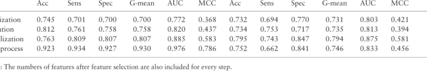
Table 2.Performance of the models of the different steps with cross-validation and on the respective test sets

Cross-validation Test Features

Step Acc Sens Spec G-mean AUC MCC Acc Sens Spec G-mean AUC MCC

Solubilization 0.745 0.701 0.700 0.700 0.772 0.368 0.732 0.694 0.770 0.731 0.803 0.421 156 Purification 0.812 0.761 0.758 0.758 0.820 0.437 0.734 0.753 0.717 0.735 0.813 0.394 193 Crystallization 0.763 0.809 0.807 0.807 0.885 0.583 0.795 0.743 0.847 0.794 0.875 0.581 201 Whole process 0.923 0.934 0.927 0.930 0.976 0.786 0.752 0.662 0.841 0.746 0.833 0.456 ––

Note: The numbers of features after feature selection are also included for every step.

Acc, Balanced accuracy; Sens, Sensitivity; Spec, Specificity and MCC, Matthew’s correlation coefficient.

Fig. 1.Performance of TMCrys. ROC curves of the performance of TMCrys both for the corresponding test sets and cross-validation. (A) Solubilization, (B) purification and (C) crystallization step. (D) Comparing the performance of TMCrys (shading: confidence interval) with existing tools for the whole process. The methods are the following: CrystalP2, XtalPred, XtalPred-RF, ParCrys, Crysalis I and Crysalis II

Table 3.Performance of the different prediction methods on the test set

Method Acc Sens Spec G-mean AUC MCC

TMCrys 0.752 0.662 0.841 0.746 0.833 0.456

Crysalis I 0.493 0.105 0.881 0.304 0.510 –0.017 Crysalis II 0.492 0.112 0.871 0.312 0.499 –0.020 XtalPred 0.491 0.016 0.967 0.124 0.482 –0.038 XtalPred-RF 0.577 0.620 0.524 0.570 0.578 0.299 CRYSTALP2 0.572 0.606 0.538 0.571 0.593 0.106 ParCrys 0.445 0.107 0.783 0.289 0.564 –0.125 Acc, Balanced accuracy; Sens, Sensitivity; Spec, Specificity and MCC, Matthews correlation coefficient.

(5)

Acknowledgements

The authors thank Andra´s Horva´th the critical reading of the manuscript and the testing of TMCrys.

Funding

This work was supported by grant K119287 from the Hungarian Scientific Research Fund (OTKA), ‘Momentum’ Program of the Hungarian Academy of Sciences (LP2012/35), FIEK_16-1-2016-0005 provided by the National Research, Development and Innovation Fund of Hungary and grant U´ NKP- 16-2_VBK-016 of the New National Excellence Programme funded by the Ministry of Human Resources.

Conflict of Interest: none declared.

References

Andre´ll,J. and Tate,C.G. (2013) Overexpression of membrane proteins in mammalian cells for structural studies.Mol. Membr. Biol.,30, 52–63.

Charoenkwan,P.et al. (2013) SCMCRYS: predicting protein crystallization using an ensemble scoring card method with estimating propensity scores of P-collocated amino acid pairs.PLoS One,8, e72368.

Chen,L.et al. (2004) TargetDB: a target registration database for structural genomics projects.Bioinformatics,20, 2860–2862.

Chen,K.et al. (2007) Prediction of protein crystallization using collocation of amino acid pairs.Biochem. Biophys. Res. Commun.,355, 764–769.

Chen,T.et al. (2017) xgboost: extreme gradient boosting (R package from CRAN; https://cran.r-project.org/web/packages/xgboost).

Chen,T. and Guestrin,C. (2016)XGBoost.In:Proceedings of the 22nd ACM SIGKDD International Conference on Knowledge Discovery and Data Mining–KDD ’16. ACM Press, New York, NY, USA, pp. 785–794.

Dobson,L.et al. (2015a) CCTOP: a Consensus Constrained TOPology prediction web server.Nucleic Acids Res.,43, W408–W412.

Dobson,L.et al. (2015b) The human transmembrane proteome.Biol. Direct, 10, 31.

Fu,L.et al. (2012) CD-HIT: accelerated for clustering the next-generation sequencing data.Bioinformatics,28, 3150–3152.

Gabanyi,M.J.et al. (2011) The Structural Biology Knowledgebase: a portal to protein structures, sequences, functions, and methods. J. Struct. Funct.

Genomics,12, 45–54.

Gubellini,F.et al. (2011) Physiological response to membrane protein overexpression inE. coli.Mol. Cell. Proteomics,10, M111.007930.

Hite,R.K. and MacKinnon,R. (2017) structural titration of Slo2.2, a Naþ-dependent Kþchannel.Cell,168, 390–399.e11.

Hopkins,A.L. and Groom,C.R. (2002) The druggable genome.Nat. Rev. Drug Discov.,1, 727–730.

Jahandideh,S.et al. (2014) Improving the chances of successful protein structure determination with a random forest classifier.Acta Crystallogr. Sect. D Biol. Crystallogr.,70, 627–635.

Kawashima,S. et al. (1999) AAindex: amino acid index database.Nucleic Acids Res.,27, 368–369.

Kobe,B.et al. (eds.) (2008)Structural Proteomics. Humana Press, Totowa, NJ.

Kozma,D.et al. (2013) PDBTM: protein Data Bank of transmembrane proteins after 8 years.Nucleic Acids Res.,41, D524–D529.

Kuhn,M. (2008) Building predictive models in Rusing thecaretpackage.

J. Stat. Software,28, 1–26.

Kuhn,M.et al. (2017) Caret: classification and regression training (R package from CRAN; https://cran.r-project.org/web/packages/caret).

Kurgan,L.et al. (2009) CRYSTALP2: sequence-based protein crystallization propensity prediction.BMC Struct. Biol.,9, 50.

Love,J.et al. (2010) The New York consortium on membrane protein structure (NYCOMPS): a high-throughput platform for structural genomics of integral membrane proteins.J. Struct. Funct. Genomics,11, 191–199.

Lundstrom,K. (2006) Structural genomics for membrane proteins.Cell. Mol.

Life Sci.,63, 2597–2607.

Martin-Galiano,A.J.et al. (2008) Predicting experimental properties of integral membrane proteins by a naive Bayes approach.Proteins Struct. Funct.

Genet.,70, 1243–1256.

Mirzadeh,K.et al. (2016)Codon Optimizing for Increased Membrane Protein Production: A Minimalist Approach. Humana Press, New York, NY, pp. 53–61.

Moraes,I.et al. (2014) Membrane protein structure determination - the next generation.Biochim. Biophys. Acta,1838, 78–87.

Nogales,E. (2016) The development of cryo-EM into a mainstream structural biology technique.Nat. Methods,13, 24–27.

Olson,R.S.et al. (2017) Data-driven advice for applying machine learning to bioinformatics problems, arXiv:1708.05070 [q-bio.QM].

Overton,I.M. and Barton,G.J. (2006) A normalised scale for structural genomics target ranking: the OB-Score.FEBS Lett.,580, 4005–4009.

Petersen,B.et al. (2009) A generic method for assignment of reliability scores applied to solvent accessibility predictions.BMC Struct. Biol.,9, 51.

Provost,F. and Fawcett,T. (2001) Robust classification for imprecise environ- ments.Mach. Learn,42, 203–231.

Saladi,S.M.et al. (2018) Decoding sequence-level information to predict membrane protein expression.J. Biol. Chem.,293, 4913–4927.

Scott,D.J.et al. (2013) Stabilizing membrane proteins through protein engineering.Curr. Opin. Chem. Biol.,17, 427–435.

Slabinski,L.et al. (2007) XtalPred: a web server for prediction of protein crys- tallizability.Bioinformatics,23, 3403–3405.

Varga,J. et al. (2017) TSTMP: target selection for structural genomics of human transmembrane proteins.Nucleic Acids Res.,45, D325–D330.

Walker,J.M.(ed) (2005)The Proteomics Protocols Handbook. Humana Press, Totowa, NJ.

Wang,H.et al. (2014) PredPPCrys: accurate prediction of sequence cloning, protein production, purification and crystallization propensity from protein sequences using multi-step heterogeneous feature fusion and selection.PLoS One,9, e105902.

Wang,H.et al. (2016) Crysalis: an integrated server for computational analysis and design of protein crystallization.Sci. Rep.,6, 21383.

Wang,H.et al. (2017) Critical evaluation of bioinformatics tools for the prediction of protein crystallization propensity.Brief. Bioinform.,7, 1–15.

Xiao,N. et al. (2015) protr/ProtrWeb: r package and web server for generating various numerical representation schemes of protein sequences.

Bioinformatics,31, 1857–1859.