Common priors for generalized type spaces ∗
Mikl´ os Pint´ er
†February 18, 2012
”Give me a place to stand on, and I will move the Earth.”
Archimedes Abstract
The notion of common prior is well-understood and widely-used in the incomplete information games literature. For ordinary type spaces the common prior is defined.
Pint´er and Udvari (2011) introduce the notion of generalized type space. Generalized type spaces are models for various bonded ratio- nality issues, for finite belief hierarchies, unawareness among others.
In this paper we define the notion of common prior for generalized types spaces.
Our results are as follows: the generalization (1) suggests a new form of common prior for ordinary type spaces, (2) shows some quan- tum game theoretic results (Brandenburger and La Mura, 2011) in new light.
Keywords and phrases: Type spaces; Generalized type spaces;
Common prior; Hars´anyi Doctrine; Quantum games JEL codes: C72, D83
1 Introduction
The common prior is a central notion of games with incomplete information since the very beginnings (Hars´anyi, 1967-68). The intuition behind the common prior is clear, it aggregates all information of the model, it works as
∗I thank M´arton Benedek for his remarks, and acknowledge the support by the J´anos Bolyai Research Scholarship of the Hungarian Academy of Sciences and grant OTKA.
†Corresponding author: Department of Mathematics, Corvinus University of Budapest, 1093 Hungary, Budapest, F˝ov´am t´er 13-15., miklos.pinter@uni-corvinus.hu.
a source of all information, that is, e.g. the players’ beliefs can be deduced from it.
For ordinary type spaces (Heifetz and Samet, 1998) the common prior is known, it grabs the same intuitions as that for finite models it gives. In type spaces the players’ beliefs are explicitly given by the so called type functions, so a common prior is a probability measure which is compatible with the players’ beliefs. This compatibility can be well-defined by the notion of conditional probability.
Pint´er and Udvari (2011) introduce the notion of generalized type space.
Generalized type spaces are models for ordinary belief hierarchies and for various bounded rationality issues, e.g. for finite hierarchies of beliefs, un- awareness among others. In other words, generalized type spaces are gener- alizations of ordinary type spaces (Heifetz and Samet, 1998), that is, every ordinary type space is a generalized type space.
In this paper we define the common prior for generalized type spaces.
The intuition is the same as for ordinary type spaces, that is, a certain compatibility with the players’ beliefs is required. Since in generalized type spaces the players’ beliefs can be very different from those in ordinary type spaces we define the common prior as a common type function, a mapping which assigns a probability measure to each state of the world, in a way such that, at each state of the world the players’ beliefs (given by the type functions) are compatible with the given probability measure. However, in generalized type spaces the players might have beliefs about very few events only, so the word compatibility means less in this case than in the case of ordinary type spaces.
In the setting of generalized type spaces compatibility means that at each state of the world each player cannot learn more or less from the common prior than that she learns from her own type function. In generalized type spaces, however, it can happen that each player knows nothing, in which case any mapping is a common prior. Therefore, the common priors can be very different for the very same generalized type space.
Technically, while in ordinary type spaces with common prior the type functions are conditional probabilities, this is not the case for generalized type spaces. In the generalized type space setting the type functions are less than conditional probabilities, so they can vary more.
A further point, in this paper we work with purely measurable gener- alized type spaces, so with a generalization of Heifetz and Samet (1998)’s type space. Even if most of the works in the literature use topological type spaces, see B¨oge and Eisele (1979); Mertens and Zamir (1985); Heifetz (1993);
Brandenburger and Dekel (1993); Mertens et al (1994); Heifetz and Samet (1999); Pint´er (2005) among others, the results of Heifetz and Samet (1998);
Pint´er (2010, 2012) tell us to prefer the purely measurable to the topological framework.
We mention two results of the paper. First, we define the common prior as a common type function. This approach fits well to the type space setting, and makes possible for us to discuss the problem in an elegant form. However, this implies also that we have to reformulate the common prior for ordinary type spaces. This reformulation does not bring new issues for ordinary type spaces, so we can say our notion of common prior is the same as the one well-known in the literature (for ordinary type spaces).
Second, our notion of common prior can interpret the quantum correla- tion ”device” e.g. in Brandenburger and La Mura (2011)’s paper. In other words, we can interpret the quantum correlation as an ordinary correlation for boundedly rational players, that is, as a common prior for generalized type spaces. In this sense, our result shows quantum game theoretic results in new light.
Finally, we give an explanation for the citation from Archimedes in the head of the paper. One of the main difference between ordinary and gen- eralized type spaces is that the ordinary type spaces are Hars´anyi type spaces, while the the generalized type spaces are not necessarily Hars´anyi type spaces, that is, in ordinary type spaces the players know their own types, while it needs not to happen in generalized type spaces. That a player knows her own type is “the place to stand on“. If this ”place” is missing, then the players can do less, but it makes possible for external factors (com- mon prior) to coordinate the players’ beliefs more subtle ways than in models where the players know their own types. Definitely, Archimedes did not mean the same by the above citation as that we do.
The setup of the paper is as follows. In the next section we introduce the notion of common prior for generalized type spaces in a finite, simple setting. In Section 3 we explain the introduced notion by examples. Section 4 is about applications of the previously discussed models. The last section briefly concludes. In an appendix we give the notion of common prior for generalized type spaces in the abstract setting.
2 Common priors for generalized type spaces
In this section we introduce the notion of common prior for generalized type spaces in the finite setting. We give the mathematically precise definitions in Appendix A.
In our model we assume that the player setN is a finite set, that is, there are finitely many players, and N0 =N ∪ {0} is for the extended player set,
where Player 0 is the nature as an extra player.
In generalized type spaces the players can have very different beliefs. For instance it can happen that at a certain state of the world a player has a belief which can be represented by a probability distribution defined on all subsets of the set of the states of the world, while at an other state of the world the player has a belief which can be represented by a probability distribution defined only on some subsets of the set of the states of the world.
First, we introduce the notion of states of the world.
Definition 1. Let the finite set Ω be the state of the states of the world and for each i ∈ N0, let Mi be a partition on Ω. Partition Mi represents Player i’s information, M0 is for the information available for the nature.
Let M=∨i∈N0Mi, that is Mis the coarsest partition among the partitions which contain partitions Mi.
The above notion is from Aumann (1999). The states of the world are the descriptions of the basic elements of the world, each point of Ω is for one specific state of the world. The partitions are for modeling the information of the players. Partition Mi gives what states Player i can distinguish (by cognition) and what she cannot. Partition M0 is for the information the model provides, but does not belong to any player. We say this is the nature’s information.
Usual in the literature that the parameters of the modeled situation, to which we also refer as the types of the nature, are given by a parameter set (Mertens and Zamir, 1985; Brandenburger and Dekel, 1993; Heifetz, 1993;
Heifetz and Samet, 1998; Pint´er, 2005, 2012). We also follow this way, and take set S as a parameter set. Moreover, we assume that S is a finite set, and each subset of S is an event.
We have already mentioned that in generalized type spaces the play- ers’ beliefs can be truncated, that is, those need not be defined at any event; we denote the class of this type of beliefs by ∆(Ω,M). Formally,
∆(Ω,M) is for all probability measures (distributions) defined on certain sub- sets of Ω, ∆(Ω,M) = {µis a probability measure defined on the field gen- erated by partition N : N is coarser than M}. If at a state of the world a player’s belief is a probability measure such that is not defined at event A ⊆ Ω, then we say that the player ignores event A (at the state of the world).
Definition 2. Let (Ω,Mi)i∈N0 be the set of the states of the world (see Definition 2). The generalized type space based on parameter space S is a tuple (S,Ω,{Mi}i∈N0, g,{fi}i∈N), where
• g : Ω → S is a mapping such that for each A ⊆ S there exists M1, M2, . . . , Mn∈ M0 ∪ {∅} such that g−1(A) = ∪nj=1Mj,
• fi : Ω→∆(Ω,M) is a mapping such that for each A⊆∆(Ω,M) there exists M1, M2, . . . , Mn ∈ Mi∪ {∅} such thatfi−1(A) =∪nj=1Mj, i∈N. Mapping g connects the set of the states of the world to the parameter set. Moreover, g preserves the information given by partition M0, that is, the g-inverse image of any event in the parameter set is expressible by the elements of partition M0 and the empty set. In other words, if two states of the world are indistinguishable by partition M0, then these points have the same g-image.
fi is the type function of Player i. The type function gives the player’s beliefs at the states of the world. fi also preserves Player i’s information, that is, if the two states of the world are indistinguishable by Player i, then those have the same fi-image.
In generalized type spaces the beliefs can vary much, the players need not be aware of all events, they might know their types or not, therefore, many things can happen. The model of generalized type spaces encompasses both Hars´anyi and non-Hars´anyi type spaces (Heifetz and Mongin, 2001) and more.
In general it can happen that at a state of the world the players’ beliefs are inconsistent, that is, the players’ beliefs are very different. This can happen basically because of two things. First, when the players have different piece of information about the state of the world, so the differences in their beliefs are due to quantity of information available for the players, in this case there is no substantial disagreement about the state of the world among the players.
Second, when the differences of the players’ beliefs are due to substantial disagreement, in other words, when the information available for the player differ in its quality not only in its quantity. Typically this happens when the players can agree to disagree on a commonly known event (Aumann, 1976).
In the first case we say the generalized type space has (a) common prior(s), in the second we say it has not.
Definition 3(Common prior for generalized type spaces). Consider general- ized type space (S,{Ω,Mi}i∈N0, g,{fi}i∈N). f : Ω→∆(Ω,M) is a common prior, if for each ω ∈Ω, i∈N, A⊆Ωsuch that fi(ω) is defined at event A:
f(ω)(A) = X
ω0∈Ω
fi(ω0)(A) f(ω)({ω0}) .
The notion of common prior formalizes the intuition we have discussed above. If there is a common prior for a generalized type space, then there is no substantial differences in the players’ beliefs, that is, those are consistent.
Remark 4. We do not discuss it in details, only mention it, that Aumann (1976)’s result holds for generalized type spaces too. Formally, for any gen- eralized type space having Common Prior, if at a state of the world event A is commonly known, then it cannot be commonly known that the players’
beliefs about event A at the state of the world do not coincide; that is, the players cannot agree to disagree.
It is also worth mentioning that the type functionsfi are not (necessarily) conditional probabilities. If type functions fi were conditional probabilities, then those should meet the following condition, for each ω ∈ Ω, i ∈ N, A, B ⊆Ω such that fi(ω) is defined at eventA, andB ∈ Mi:
f(ω)(A∩B) = X
ω0∈B
fi(ω0)(A) f(ω)({ω0}) . (1) The difference is obvious, if A∩B =∅, then the conditional probability must be 0 (f(ω)(B)>0,fi(ω0)(A), ω0 ∈B in (1)), while this is not the case in (3). In other words, since the generalized type spaces are not (necessarily) Hars´anyi type spaces, the type functions are not (necessarily) conditional probabilities.
3 Examples
In this section we provide two examples for illustrating the notions introduced in the previous section. The first example is about an ordinary Hars´anyi type space.
Example 5. Take generalized type space (S,{Ω,Mi}i∈N0, g,{fi}i∈N), where
• N ={1,2},
• S ={∗},
• Ti ={t1i, t2i}, i∈N,
• Ω = S×T1×T2,
• M0 ={Ω}, Mi ={{∗} × {t1i} ×T−i,{∗} × {t2i} ×T−i},i∈N,
• for each Player i ∈ N and state of the world ω = (∗, ti, t−i) ∈ Ω:
fi(ω) is defined at each subset of Ω, and fi(ω)({∗} × {ti} × {t1−i}) = fi(ω)({∗} × {ti} × {t2−i}) = 12 .
This type space is a Hars´anyi type space, that is, each player knows her own type, more precisely, each player believes with probability 1 her own type, and at each state state of the world, each player’s belief is defined on M, that is, each player is aware of, so can form beliefs about, any event.
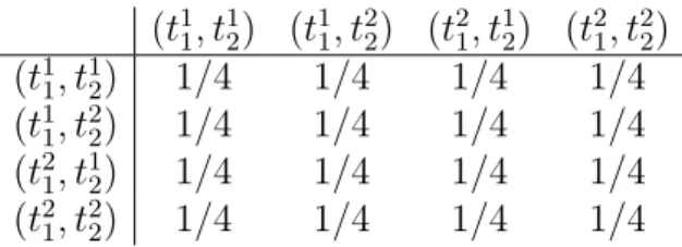
Take state of the world ω = (∗, t1, t2)∈ Ω. If f is a common prior, then f(ω)({∗} × {t1} × {t2}) = f(ω)({∗} × {t1} ×T2\ {t2}) = f(ω)({∗} ×T1\ {t1} × {t2}) = f(ω)({∗} ×T1\ {t1} ×T2\ {t2}). So the unique common prior has the same value at each state of the world, see Table 1 (we do not put the state of the nature in the model, because that does not count).
(t11, t12) (t11, t22) (t21, t12) (t21, t22) (t11, t12) 1/4 1/4 1/4 1/4 (t11, t22) 1/4 1/4 1/4 1/4 (t21, t12) 1/4 1/4 1/4 1/4 (t21, t22) 1/4 1/4 1/4 1/4
(2)
Table 1: The common prior for the Hars´anyi type space of Example 5 Therefore, in this example we have got a ”classical” common prior, that is, we can use a unique distribution, see Table 2.
T1\T2 t12 t22 t11 1/4 1/4 t21 1/4 1/4
Table 2: The “classical“ common prior for the Hars´anyi type space of Ex- ample 5
In the above example we have seen that in certain cases the common prior has the same value at each state of the world, put it differently, we can say that the common prior is a probability distribution (measure) on the set of the states of the world. In the following proposition we formalize this observation, but first, we introduce a notion.
Definition 6. Consider generalized type space (S,{Ω,Mi}i∈N0, g,{fi}i∈N) such that it has a common prior f. For each state of the world ω ∈ Ω let undirected graph (Vω, Eω) be defined as Vω ={B ∈ ∪i∈NMi :f(ω)(B)>0}, and BB0 ∈Eω, if there exist A, A0 ∈ ∨i∈N0Mi and B00 ∈ ∪i∈N0Mi such that A⊆B ∩B00, A0 ⊆B0∩B00, and f(ω)(A), f(ω)(A0)>0.
Now, we can provide the above mentioned proposition.
Proposition 7. Take generalized type space(S,{Ω,Mi}i∈N0, g,{fi}i∈N)such that
1. it has a common prior f,
2. fi(ω) is defined at each event A ∈ ∨i∈N0Mi, ω∈Ω, i∈N, 3. for each B ⊆ Mi, ω ∈B: fi(ω)(B) = 1, ω∈Ω, i∈N.
Then for each states of the world ω, ω0 ∈ Ω such that there exists B∗ ∈
∧i∈NMi such that 4. ω, ω0 ∈B∗,
5. both (Vω∩B∗, Eω) and (Vω0∩B∗, Eω0) are connected undirected graphs, f(ω) = f(ω0) .
Proof. From Points 1., 2., 3. and 4. for each Player i∈N: fi(ω)(B∗) = 1.
Let A ∈ ∨i∈N0Mi be such that A ⊆ B∗ and f(ω)(A) > 0. Then for each A0 ∈ ∨i∈N0Mi such that there exists Playeri ∈N, Bi ∈ Mi such that A, A0 ⊆Bi:
f(ω)(A) = X
ω0∈Ω
fi(ω0)(A)f(ω) = X
ω0∈Bi
fi(ω0)(A)f(ω) =fi(ωBi)(A)f(ω)(Bi), similarly,
f(ω)(A0) = X
ω0∈Ω
fi(ω0)(A0)f(ω)
= X
ω0∈Bi
fi(ω0)(A0)f(ω) =fi(ωBi)(A0)f(ω)(Bi) , where ωBi ∈Bi.
Since f(ω)(A)>0,f(ω)(Bi)>0 and fi(·)(A)>0:
f(ω)(A0)
f(ω)(A) = fi(·)(A0) fi(·)(A) ,
that is, f(ω)(Af(ω)(A)0) is given by the generalized type space (by fi).
Since (Vω∩B∗, Eω) is connected (Point5.), for eachA0 ∈ ∨i∈N0MiA0 6=A,
f(ω)(A0)
f(ω)(A) is given (if A * B, then ff(ω)(A(ω)(A)0) = 0). Furthermore, we have the equations: f(ω)(A0) =fi(ωBi)(A)f(ω)(Bi), as many as | ∨i∈N0 Mi| −1 (the
number of atoms minus 1), and equation PA0∈∨i∈N
0Mif(ω)(A0) = 1; these equations are (linearly) independent; moreover we have as many as|∨i∈N0Mi| unknowns (the probabilities f(ω)(A0) and f(ω)(A)), so f(ω) is well-defined, that is, it is uniquely determined by the generalized type space (by the type functions).
Similarly, the above argument can be applied to f(ω0), so f(ω0) is well-
defined too, therefore f(ω) =f(ω0).
In the second example the common prior is neither “classical“ nor unique.
Example 8. Take generalized type space (S,{Ω,Mi}i∈N0, g,{fi}i∈N), where
• N ={1,2},
• S ={∗},
• Ti ={t1i, t2i}, i∈N,
• Ω = S×T1×T2,
• M0 ={Ω}, Mi ={{∗} × {t1i} ×T−i,{∗} × {t2i} ×T−i},i∈N,
• for each Player i ∈ N and state of the world ω ∈ Ω: fi(ω) is defined only onMi, andfi(ω)({∗} × {t1i} ×T−i) = fi(ti)({∗} × {t2i} ×T−i) = 12, i∈N.
Then it is a slight calculation to see that the mapping given in Table 1 is a common prior for this type space. However, so is the mapping given in Table 3 (this numerical example is from Abramsky and Brandenburger (2011)).
(t11, t12) (t11, t22) (t21, t12) (t21, t22) (t11, t12) 3/8 1/8 1/8 3/8 (t11, t22) 1/8 3/8 3/8 1/8 (t21, t12) 3/8 1/8 1/8 3/8 (t21, t22) 1/8 3/8 3/8 1/8
(3)
It is worth noticing that the two common priors provided in Example 8 are very different. The first one (Table 1) can be interpreted as there is no relation among the states of the world, however, the second (Table 3) shows a very subtle and smart relation among the states of the world.
4 Applications
By generalized type spaces we can model finite belief hierarchies, unaware- ness, and other various phenomena of bounded cognitive abilities (Pint´er and Udvari, 2011). In the “classical” models the common prior is a tool of coor- dination. By common priors the players, more precisely, the players’ beliefs, can be harmonized, so that the outcome of the game can Pareto outperform the outcomes achievable without harmonization (Aumann, 1974, 1987).
For generalized type spaces the common prior can harmonize the players’
beliefs in smarter ways than that classical common priors do. This smarter harmonization allows outcomes to Pareto outperform those achieved by clas- sical harmonizations.
Perhaps, the key point in general type spaces is that the players need not know their own types. From the viewpoint of mathematics, it is not difficult to formalize and handle this. However, it could be difficult to give a good decision theoretic interpretation for this type of cognitive incapability of the players.
We demonstrate our decision theoretic interpretation by the example of the Prisoner’s Dilemma.
Example 9. Consider the following 2×2 strategic form game:
• N ={1,2} is the player set,
• Ai ={C, D} are the action sets,i∈N,
• the payoffs, which depend on the players’ types are in Table 3.
Player 2
D C
Player 1 D C
(13,13) (15,0)
(0,15) (11,11) Table 3: The payoffs of Example 9
The considered game is a classical Prisoner’s Dilemma game, so the only correlated (Nash equilibrium) is the strategy profile (C, C). By applying the notion correlated equilibrium (Aumann, 1987) implicitelly we take types and type spaces, so we must formally give the type space we consider. First we give only the backbone of the type space.
Take generalized type space (S,{Ω,Mi}i∈N0, g,{fi}i∈N), where
• S ={∗}is the parameter set,
• Ti ={t1i, t2i} are the type sets, i∈N,
• Ω = S×T1×T2 is the set of the states of the world.
We have not specified yet the information and the type functions of the players, we do it later. However, it is clear from the above given details, that we consider a complete information situation, and again the only correlated and (Bayesian) Nash equilibrium is that where both players always play C (confess). In other words, whatever ordinary common prior we put in the above type space we cannot achieve better equilibrium payoffs than (11,11).
Now, consider the following ingredients which are missing from the gen- eralized type space above:
• M0 ={Ω}, Mi ={{∗} × {t1i} ×T−i,{∗} × {t2i} ×T−i}, i∈N are the (information) partitions,
• for each Playeri∈N and state of the world ω∈Ω: fi(ω) is defined on the field induced byMi, andfi({∗}×{t1i}×T−i)({∗}×{t1i}×T−i) = 0.7, fi({∗} × {t2i} ×T−i)({∗} × {t1i} ×T−i) = 0.5,
• take the common prior of Table 4.
(t11, t12) (t11, t22) (t21, t12) (t21, t22) (t11, t12) 0.7 0 0 0.3 (t11, t22) 0.4 0.3 0.1 0.2 (t21, t12) 0.4 0.1 0.3 0.2 (t21, t22) 0 0.5 0.5 0
(4)
Table 4: The common prior of Example 9.
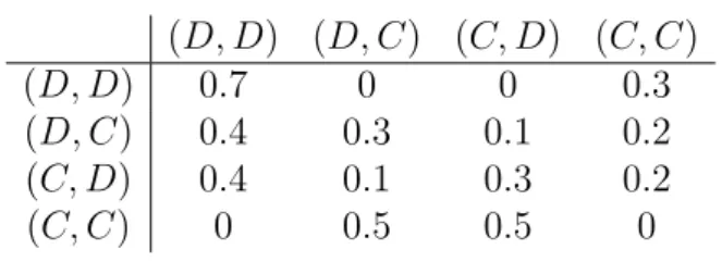
Next, we follow Aumann (1987) and take an ”outside observer” perspec- tive. We assume that t1i means the player takes actionD, and t2i means she takes action C, i∈N. Then we get the common prior of Table 5.
The interpretation is as follows: the first row means, if both players play actionD,then outcome (D, D) happens with probability 0.7, (C, C) happens with probability 0.3, and the other outcomes happen with probability 0. The other rows can be interpreted in the same way.
According to the common prior of Table 5, at each state each player believes that whatever action she takes her real action is D and C with
(D, D) (D, C) (C, D) (C, C)
(D, D) 0.7 0 0 0.3
(D, C) 0.4 0.3 0.1 0.2
(C, D) 0.4 0.1 0.3 0.2
(C, C) 0 0.5 0.5 0
(5)
Table 5: The common prior of Example 9.
certain probability (depending on the states of the world). Moreover, no player has beliefs about the other players’ actions.
Next, we show that in this game (D, D) is a “generalized correlated equi- librium”. First, see the players’ expected payoffs (Table 6) given by the common prior.
The payoffs (D, D) (12.4,12.4) (D, C) (8.9,11.9) (C, D) (11.9,8.9) (C, C) (7.5,7.5)
(6)
Table 6: The payoffs of Example 9.
Then, it is clear from Table 6 that the unique (dominant) equilibrium is (D, D), since if a player unilaterally deviates, then she gets 11.9 instead of 12.4 and 7.5 instead of 8.9 in cases of the other player takes actions D and C respectively.
Putting a story behind the common prior of Table 5, assume that con- fessing is very risky it succeeds only in the half of the cases, because no prisoner is sure in that she is able to give really useful information to the authorities, e.g. she is not sure in that the information, she can provide, is enough against the other prisoner. In other words, the players cannot confess for sure, only with probability half. However, the players are more successful in denying, it succeeds in 70% of the cases, in the other cases the prisoner breaks down and confesses. The “hidden correlation“ is interpreted as the lawyers’ ”contribution”.
We mention two further applications, interpretations of our common prior concept. The first one is Brandenburger and La Mura (2011)’s, who consider one player games in extensive form. If a game does not meet the property of perfect recall, then there are decision points indistinguishable by the player, that is, the decision points are in the same information set, and those are
different only in the player’s previous moves. This setting can be modeled as the player does not know her previous moves, that is, she does not know her own strategy, which is equivalent with that she knows her strategy, but does not her type. In other words, generalized type space can be good frameworks for this kind of problems too.
Usually, the description of incomplete information models starts with that the players learn their own types. In many cases, however, this is not realistic. For instance, many people evaluate their own physical and mental strength wrong. Many times we hear sentences like “I had thought I was strong enough, but I was not“. Considering these uncertainties, and putting them into a model, we get generalized type spaces.
Filar and Beck (2007)’s model is an other approach. In their model the players’ incompetence makes that the players’ control over their actions is not 100%, that is, even if a player intends to take a certain action, she plays a different, maybe mixed, action. Filar and Beck (2007)’s approach is similar to the trembling-hand models, but not the same. In their model the players know their incapability of playing the exact action, and they decide by using this knowledge (an other difference is that in Filar and Beck (2007) the hand can tremble in strange and not uniform ways too).
Therefore, putting Filar and Beck (2007)’s idea in the incomplete informa- tion setting, the players know their own types, but not their own strategies.
However, this is equivalent with that, the players know their own strategies but not their own types. That is, we get generalized type spaces again.
Finally, notice that in Example 9 both above mentioned approaches are present. The example can interpreted as either a model where the players cannot know their types or a framework where the players cannot control their own actions perfectly.
5 Conclusion
In this paper we have introduced the notion of common prior for generalized type spaces. We have showed that a generalized type space can be compatible with substantially different common priors.
Moreover, for generalized type spaces the common priors can harmonize the players’ beliefs on very different levels. In Example 8 one of the two common priors gives no harmonization at all (see Table 1), while the other (see Table 3) provides a very smart harmonization of the players’ beliefs.
This phenomenon rises substantial decision theoretical questions.
Example 8 clearly shows that the common prior can be more than the
”sum” of the players’ information (Pint´er (2011) concludes the same on a
different basis). Therefore, in certain cases generalized type spaces are not complete descriptions of decision theoretic situations. This, again, shows that it is not enough to take account of the players’ beliefs (generalized type spaces), the relation of their beliefs should be also considered (common prior).
Furthermore, Example 9 indicates that equilibria in models by generalized type spaces with common prior can Pareto-outperform ordinary correlated equilibria (naturally so can it Nash equilibria). This can happen, because by generalized type spaces with common prior we can reproduce (certain) quantum game theory results.
A Common prior – the abstract model
In this section we give the mathematically precise definitions of the notions used in the paper. We do not give interpretations, the reader can find those in the main text and in Pint´er and Udvari (2011).
Notations: Let N be the set of the players, w.l.o.g. we can assume that 0∈/ N, and let N0 =N ∪ {0}, where 0 is for the nature as a player.
For any set systemA ⊆ P(X): σ(A) is the coarsestσ-field which contains A.
First we introduce the notion of generalized type space. We generalize or- dinary type spaces, and use terminologies, notions similar to those of Heifetz and Samet (1998).
Definition 10. Let X be a space, M be a class of σ-fields on set X and
∆(X,M) be the class of probability measures on the σ-fields of M, formally
∆(X,M) = {µ∈ ∆(X,M) :M ∈M}. Then the σ-field A∗ on ∆(X,M) is defined as follows:
A∗ =σ({{µ∈∆(X,M) :µ(A)≥p}, A ∈ M, p∈[0,1]}) .
In other words, A∗ is the smallest σ-field among the σ-fields which contain the sets {µ ∈∆(X,M) :µ(A) ≥ p}, where M ∈ M, A ∈ M and p ∈ [0,1]
are arbitrarily chosen.
Notice thatA∗ is not a fixed σ-field, we mean, it depends on the measur- able spaces on which the probability measures are defined.
Assumption 11. Let the parameter space (S,A) be a measurable space.
Henceforth we assume that (S,A) is a fixed parameter space which con- tains all states of the nature. We can think of S as a set which encompasses all the not commonly known parameters of the considered situation.
Definition 12. Let Ω be the space of the states of the world and for each i ∈ N0: let Mi be a σ-field on Ω. The σ-field Mi represents Player i’s information, M0 is for the information available for the nature, hence it is the representative of A, the σ-field of the parameter space S. Let M = σ(∪i∈N0Mi), the smallest σ-field which contains σ-fields Mi.
For the sake of brevity, henceforth – if it does not make confusion – we do not indicate the σ-fields. E.g. instead of (S,A) we write S, or ∆(S) instead of (∆(S,A),A∗). However, in some cases we refer to the non-written σ-field: e.g. A ∈ ∆(X,M) is a set of A∗, that is, it is a measurable set in the measurable space (∆(X,M),A∗), but A ⊆ ∆(X,M) keeps its original meaning: A is a subset of ∆(X,M).
Definition 13. Let (Ω,{Mi}i∈N0) be a space of the states of the world (see Definition 12). The generalized type space based on the parameter space S is a tuple (S,Ω, {Mi}i∈N0, g,{fi}i∈N), where
1. g : Ω→S is M0-measurable,
2. fi : Ω→∆(Ω,M) is Mi-measurable, i∈N, where M={N is a σ-field on Ω :N ⊆ M}.
The generalized type spaces are not Hars´anyi type spaces (Heifetz and Mongin, 2001), that is, the players do not necessarily know their own types, more precisely, they do not necessarily believe with probability 1 their own types.
Definition 14 (Common prior for generalized type spaces). Consider gen- eralized type space (S,{(Ω,Mi)}i∈N0, g,{fi}i∈N). f : Ω → ∆(Ω,M) is a common prior, if for each ω ∈ Ω, i ∈ N, A ∈ M such that fi(ω) is defined at event A:
f(ω)(A) =
Z
Ω
fi(·)(A) df(ω) .
The common prior is a ”universal” type function, a type function which summarizes the beliefs of all the players at each state of the world. In other words, by a common prior the differences in the player’s beliefs are due to the quantity of information and not to the quality of the information available to the players.
References
Abramsky S, Brandenburger A (2011) The sheaf-theoretic structure of non- locality and contextuality, manuscript
Aumann RJ (1974) Subjectivity and correlation in randomized strategies.
Journal of Mathematical Economics 1:67–96
Aumann RJ (1976) Agreeing to disagree. The Annals of Statistics 4(6):1236–
1239
Aumann RJ (1987) Correlated equilibrium as an expression of bayesian ra- tionality. Econometrica 55(1):1–18
Aumann RJ (1999) Interacitve epistemology i: Knowledge. International Journal of Game Theory 28:263–300
B¨oge W, Eisele T (1979) On solutions of bayesian games. International Jour- nal of Game Theory 8(4):193–215
Brandenburger A, Dekel E (1993) Hierarchies of beliefs and common knowl- edge. Journal of Economic Theory 59:189–198
Brandenburger A, La Mura P (2011) Quantum decision theory, manuscript Filar J, Beck J (2007) Games, Incompetence and Training, Annals of the
International Society of Dynamic Games, vol 9, Springer, pp 93–110 Hars´anyi J (1967-68) Games with incomplete information played by bayesian
players part i., ii., iii. Management Science 14:159–182, 320–334, 486–502 Heifetz A (1993) The bayesian formulation of incomplete information - the
non-compact case. International Journal of Game Theory 21:329–338 Heifetz A, Mongin P (2001) Probability logic for type spaces. Games and
Economic Behavior 35(1-2):31–53
Heifetz A, Samet D (1998) Topology-free typology of beliefs. Journal of Eco- nomic Theory 82:324–341
Heifetz A, Samet D (1999) Coherent beliefs are not always types. Journal of Mathematical Economics 32:475–488
Mertens JF, Zamir S (1985) Formulation of bayesian analysis for games with incomplete information. International Journal of Game Theory 14:1–29
Mertens JF, Sorin S, Zamir S (1994) Repeated games part a. CORE Discus- sion Paper No 9420
Pint´er M (2005) Type space on a purely measurable parameter space. Eco- nomic Theory 26:129–139
Pint´er M (2010) The non-existence of a universal topological type space.
Journal of Mathematical Economics 46:223–229
Pint´er M (2011) A note on the common prior, manuscript
Pint´er M (2012) Every hierarchy of beliefs is a type URL http://arxiv.
org/abs/0805.4007, arXiv0805.4007v3
Pint´er M, Udvari Z (2011) Generalized type spaces, mPRA Paper No. 34107