A. Rácz, D. Bajusz & K. Héberger, Modelling methods and cross-validation variants in QSAR: a multi-level analysis$
SAR and QSAR in Environmental Research
http://dx.doi.org/10.1080/1062936X.2018.1505778
Received 11 Jul 2018, Accepted 24 Jul 2018, Published online: 30 Aug 2018
Proceedings of the 18th International Conference on QSAR in Environmental and Health Sciences (QSAR 2018)
Modeling methods and cross-validation variants in QSAR modeling:
A multi-level analysis
Anita Rácz1, Dávid Bajusz2, Károly Héberger1,*
1 Plasma Chemistry Research Group, Research Centre for Natural Sciences, Hungarian Academy of Sciences, H-1117 Budapest XI., Magyar tudósok körútja 2, Hungary
2 Medicinal Chemistry Research Group, Research Centre for Natural Sciences, Hungarian Academy of Sciences, H-1117 Budapest XI., Magyar tudósok körútja 2, Hungary
*Corresponding author: Károly Héberger (heberger.karoly@ttk.mta.hu)
Abstract
Prediction performances often depend on the applied cross- and test validation protocols as well. Several combination of different cross-validation variants and model building techniques were used to reveal their complexity. Two case studies (acute toxicity data) were examined, applying five-fold cross-validation (with random, contiguous and Venetian blind forms) and leave- one-out cross-validation (CV). External test sets showed the effects and differences amongst the validation protocols. The models were generated with multiple linear regression (MLR), principal component regression (PCR), partial least squares (PLS) regression, artificial neural networks (ANN) and support vector machines (SVM). The comparisons were made by sum of ranking differences (SRD) and factorial ANOVA.
The largest bias and variance could be assigned to the MLR method and contiguous block cross-validation. SRD can provide a unique and unambiguous ranking of methods and CV variants.
Venetian blind cross-validation is a promising tool. The generated models were also compared based on their basic performance parameters (R2 and Q2). MLR produced the largest gap, while PCR gave the smallest. Although PCR is the best validated balanced technique, SVM always outperformed the other methods, when experimental values were the benchmark. Variable selection was advantageous, and the modeling had a larger influence than CV variants.
Keywords: QSAR, toxicity, validation, SRD, cross-validation, MLR, PLS, PCR, SVM, ANN
Introduction
Quantitative structure-activity (toxicity, property, etc.) relationships (abbreviated as QSAR, QSTR, QSPR, etc.) occupy a paradoxical status in the toolbox of computational chemistry. On one hand, they are one of the oldest approaches to predicting molecular properties, dating back to the work of Hansch and Fujita in the sixties (QSAR) [1,2], and even further back to the approach of Hammett to describe the equilibrium and rate constants for many reactions involving benzoic acid derivatives in the thirties (QSPR) [3]. As a consequence, these approaches had several decades, along with a large popularity among the scientific community to be refined and matured, and indeed, with the immense computational speed-up of the past decades, building QSAR models have become a routine task by the present day.
On the other hand, for the very same reason, many alternatives have emerged to each of the sub- tasks associated with QSAR modeling (including molecular descriptor calculation, variable selection, model building and validation), resulting in endless possibilities to realize the generation and selection of QSAR models. In the lack of intention to recapitulate the evolution of QSAR, we simply point the reader’s attention to two works overviewing the QSAR field: the landmark book of Hugo Kubinyi [4] and a recent review from an international team of the acknowledge experts of the field [5]. Since the abbreviations QSAR, QSTR, etc. are merely formal notations of the modeled property (A for activity, T for toxicity, etc.) without a difference in the methodology itself, we will use the abbreviation QSAR as an umbrella term for any computational task aimed at the modeling of a molecular property based on other molecular properties.
Two sub-areas of QSAR modeling with particularly thriving discussions in the relevant literature is the descriptors used for QSAR models (especially the application of 2D vs. 3D descriptors [6]), and the validation practices recommended or preferred in such studies (especially cross-validation vs. external validation [7]). 3D-QSAR is a wide collection of ligand-based (e.g. CoMFA [8]) and receptor-based methods that utilize descriptors encoding information about the 3D structure of the ligands or their protein targets [9]. While the concept is successfully applied even to the present day [10], it has also received criticism over the years [11]. Similarly, validation practices are highly debated with some authors advocating external validation as the true measure of predictive performance [12,13], while others argue that cross-validation is superior to hold-out samples [14,15]. Recently, we have contributed to this discussion by systematic comparisons of various performance parameters calculated based on cross- and external validation [16,17]. Briefly, our
results have highlighted the importance of cross-validation based performance metrics, which generally provide a more reliable assessment of the overall performances of QSAR models (in comparison to external validation-based performance metrics), as demonstrated by SRD-based comparisons. Additional works to note are the instructional paper of Dearden et al. on the common pitfalls of QSAR modeling [18], the recent article of Hanser et al. on the very important, but somewhat subjective concept of the applicability domain [19] and a historical overview of QSAR validation parameters by Gramatica and Sangion [20].
According to the relevant literature [21,22] at least five-seven techniques should be evaluated for a fair method comparison study. Sources with less comparisons are abundant for example: [23- 25]. QSAR model building can be realized by a number of regression (MLR, PCR, PLS) and machine learning (SVM, ANN) methods.
In this work, we have carried out an analysis on the effects of the chosen modeling and validation methods on the same QSAR modeling task. Based on two case studies of toxicity datasets, we have identified the significant factors with our established combination of SRD and ANOVA analyses [26], and suggest best practices for QSAR modeling and validation.
Materials and methods Dataset preparation
Two published QSAR datasets were used for the evaluations: a toxicological study by Bertinetto and coworkers (Case study 1) [27] and a bigger toxicology dataset provided by Casotti and coworkers (Case study 2) [28]. In case study 1 the toxicity values were expressed as acute toxicities (negative base 10 logarithm of 96 h LC50, or pLC50) for the fathead minnow (Pimephales promelas), in case study 2 the predictions were carried out for acute aquatic toxicities towards Daphnia Magna (48 h LC50 data). The training and test (external) set splitting was applied as in the original studies without any modifications. For case studies 1 and 2, 51 and 435 samples were used as training, and 18 and 110 samples were used as external test sets, respectively. With the use of the original molecular structures, two sets of molecular descriptors were generated for each dataset: the complete descriptor sets of QikProp (51) [29], and of RDKit (117) [30]: in total, 168 descriptors. Highly correlated (R2 > 0.999) and constant descriptors were removed from the analysis.
Regression analysis
For modeling, PLS toolbox and MATLAB were used [31]. Five modeling methods were applied, from the commonly used multiple linear regression (MLR), principal component regression (PCR), partial least squares regression (PLS) methods to the more complex machine learning techniques such as support vector machines (SVM) and artificial neural networks (ANN). The aforementioned MLR, PCR and PLS are linear methods, where the parameters to be optimized are the vector b of regression coefficients. Thus, these techniques can be considered more robust compared to the more complex ones. On the other hand, SVM and ANN have additional regularization (or meta) parameters, which need to be optimized, such as the value of Gamma and C in the case of SVM, or the number of hidden layers and nodes in the case of ANN. For SVM, automatic grid selection was used based on the heat map plot generated by PLS Toolbox. The architecture of ANN has been selected to contain one hidden layer with one hidden node.
For data pretreatment, autoscaling was used for the X matrices and mean centering for the Y vector in each case; latent variable selection was carried out based on the first local minimum of the root mean squared error of cross-validation (RMSECV) or in the case of a missing minimum (for the first ten components), the start of the plateau was used. The models were built with variable selection and without any variable selection as well. For variable selection, an automated version implemented in PLS Toolbox was used, which is based on the calculation of variable importance in projection (VIP) and selectivity ratios (SR) together.
Fivefold cross validation with a) randomized (with twenty iterations), b) Venetian blind and c) contiguous blocks, in addition to d) leave-one-out cross-validation was applied and compared for each method. The different types of validations are summarized in Figure 1From the four types of cross-validation, leave-one-out can be the most controversial, because in combination with some methods (particularly with ANN), it can cost a very long processing time compared to the other variants, in case of many samples (n > 100).
Figure 1. Cross-validation variants on the example of three-fold cross-validation: a) random selection; b) Venetian blinds; c) contiguous blocks (i.e. stratified); d) leave-one-out [32].
Reproduced by permission of The Royal Society of Chemistry.
It should be noted that the literature is not unambiguous (uniform) in terms of how each variant is called. We distinguish k-fold and leave-many-out cross-validation, in the sense that the latter allows repeated resampling ((𝑛𝑘) combinations), whereas k-fold CV utilizes k approximately equal parts of the original data set. The latter also called Monte Carlo resampling or bootstrap.
Comparison of models
Sum of (absolute) ranking differences (SRD) with Analysis of Variance (ANOVA) was used for the comparison of the regression models. SRD is a relatively novel and simple method to compare methods, models, or any type of variables (arranged in columns) in our matrices [33,34]. It gives a fair comparison, with the use of a gold standard (e.g. reference values) or generated references such as the average, minimum of maximum values of the rows according to the features of the input matrix. The process was clearly summarized in our recent work [35] with a video slide show, but the basic steps are summarized here for clarity and easy understanding: i) first the original matrix has to have the variables to be compared in the columns and the samples (compounds) in the rows; ii) the reference (measured or generated) should be added to the matrix (as the last column); iii) the ranks are assigned in increasing magnitude for each column (including the reference); iv) the absolute differences are calculated between the reference’s ranks and the ranks of each variable; v) the sums of the absolute ranking differences (SRD values) are calculated for each column separately. The smaller the SRD values, the better, i.e. the given method, or variant is closer to the benchmark experimental (or calculated) reference. SRD has a complete double validation protocol as well. SRD values are also calculated in a normalized scale (between 0 and 100), because this way the input matrices with different numbers of rows can be compared to each
other. Randomization test is also implemented and the Gaussian-like distribution of random numbers is plotted with the given SRD values together.
Uncertainties are calculated to SRD values by a bootstrap-like cross-validation: a randomized repeated resampling; approximately one fifth of the rows of the input matrix is left out randomly and with replacement five times and the SRD procedure is repeated on the remaining (approximately) 4/5th, the whole process is repeated ten times. This type of bootstrap-like cross- validation should not be confused with the cross-validation options for model building.
In our study the gold standard reference has been selected as the original, measured toxicity values.
Additionally, we have repeated the comparisons with the use of the average values as the reference (consensus), as this choice cancels out some of the systematic and random errors that are present in the experimental values (according to the maximum likelihood principle we are better off using the average than any of the individual observation). These comparisons gave almost the same results and are reported in the Supplementary information.
Five-split bootstrap cross-validation was used with random ten outcomes, and these ten repetitions made a factorial ANOVA possible.
Factorial ANOVA decomposed the SRD values (ten values for each regression model) into three factors: i) types of cross-validations (4 levels, contiguous blocks, leave-one-out, randomized and Venetian blind denoted by CON, LOO, RND VEN, respectively); ii) use of variable selection (2 levels, yes or no); iii) types of regression methods (“methods”, 5 levels, multiple linear regression, artificial neural network, principal component regression, partial least squares regression, and support vector machine, denoted by MLR, ANN, PCR, PLS, and SVM, respectively). With ANOVA, we can establish which of these factors affect the SRD values significantly (at a given probability level).
Results and discussion
Comparison based on R2 and Q2 values
The definitions of the determination coefficient and its cross-validated counterpart:
𝑅2 = 1 −∑ (𝑦𝑖−𝑦̂𝑖)2
𝑛 𝑖=1
∑𝑛𝑖=1(𝑦𝑖−𝑦̅)2 (1)
𝑄𝐿𝑀𝑂2 = 1 −∑ ∑ (𝑦𝑖−𝑦̂𝑖/𝑗)
𝑛 2 𝑖=1 𝑚 𝑗=1
∑𝑛𝑖=1(𝑦𝑖−𝑦̅)2 (2)
In eqs. (1) and (2), 𝑦𝑖 is a single experimental value, 𝑦̅ is the mean of experimental values, 𝑦̂𝑖 is a single predicted value, 𝑦̂𝑖/𝑗 is the predicted value for the ith sample when the jth part of the dataset is left out from the training (the whole dataset is split into m parts), n is the number of samples, and i is the sample index.
The differences of these performance parameters were evaluated in the first step for both case studies. All in all, 40 models were built for Case study 1 and 36 for Case study 2. (Four models with leave-one-out cross-validation in the case of neural networks were excluded due to the very long processing times.) The R2 and Q2 values were plotted for Case study 1 and 2 in Figures 2a and 2b. Box and whisker plots were produced for each method, showing the previously mentioned performance parameters.
Figure 2. Box & whisker plots of the R2 and Q2 values for model building methods (A for Case study 1 and B for Case study 2). Median was used as the center points (boxes), the rectangles contain 50% of the data (first and third quartile) and the whiskers are located at the minimum and maximum values.
Here, the gap between the R2 and Q2 values is the most important in comparing the modeling methods: a larger gap means worse performance. A large enough gap reveals one or more influential points (outliers)[36].
It is clear that the validation performance of MLR in both case studies is quite poor, and that PCR and PLS are more robust, although they have smaller R2 and Q2 values, than SVM and ANN.
Neural networks were very unreliable based on the performance parameters. SVM also provided somewhat debatable, but more reliable and better results than ANN in both cases. Thus, judging from the performance parameters, MLR is not a wise choice for regression model building, whereas the other methods are naturally grouped based on being linear or non-linear.
Comparison based on SRD values for case study 1
SRD values were calculated for each model in the two case studies based on the predicted values of the internal and external validation samples together. In this way we could implement the possible error of both validation types and exclude the overoptimistic choice between the models.
Normalized SRD values were used to the further evaluations in ANOVA for each case. A typical example of an SRD plot can be seen in Figure 3.
Figure 3. SRD plot comparing the models of Case study 1. Normalized SRD values are shown on the y axis and the distance of the columns from the origin (which is also their height) represents their distance from the vector of reference values. The cumulative probability curve shows the cumulative distribution of SRD values for random ranking: any method overlapping with this curve (here, model 40) is not significantly better than the use of random numbers.
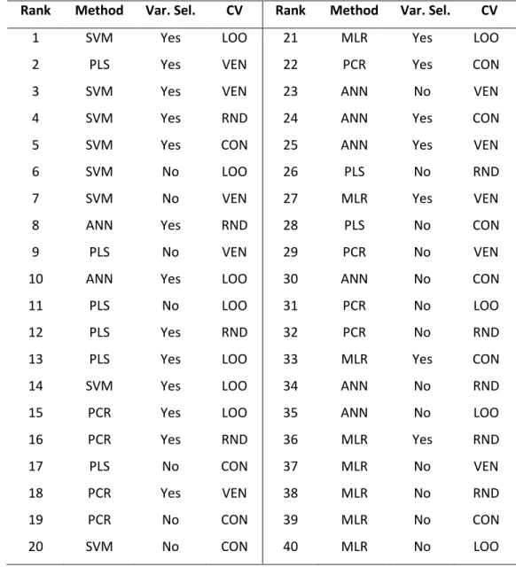
The model codes for the figure are summarized in Table 1.
Table 1. The codes for the models in Figure 3. (Var. Sel.: variable selection, CV: cross- validation.) The abbreviations for CV variants are the same as in the text.
Rank Method Var. Sel. CV Rank Method Var. Sel. CV
1 SVM Yes LOO 21 MLR Yes LOO
2 PLS Yes VEN 22 PCR Yes CON
3 SVM Yes VEN 23 ANN No VEN
4 SVM Yes RND 24 ANN Yes CON
5 SVM Yes CON 25 ANN Yes VEN
6 SVM No LOO 26 PLS No RND
7 SVM No VEN 27 MLR Yes VEN
8 ANN Yes RND 28 PLS No CON
9 PLS No VEN 29 PCR No VEN
10 ANN Yes LOO 30 ANN No CON
11 PLS No LOO 31 PCR No LOO
12 PLS Yes RND 32 PCR No RND
13 PLS Yes LOO 33 MLR Yes CON
14 SVM Yes LOO 34 ANN No RND
15 PCR Yes LOO 35 ANN No LOO
16 PCR Yes RND 36 MLR Yes RND
17 PLS No CON 37 MLR No VEN
18 PCR Yes VEN 38 MLR No RND
19 PCR No CON 39 MLR No CON
20 SVM No CON 40 MLR No LOO
The use of variable selection, CV variants and modeling methods were used as factors for ANOVA. SRD analysis was performed with the original experimental values (toxicity values) and the average as the reference, as well. With the experimental values we can choose those models and combinations of parameters which led to the best predictions of the original experimental values. On the other hand, the use of average could show us the most consistent models. On Figure 4 the averages of normalized SRD values are plotted based on the different factors in Case
study 1. Ten randomly picked SRD values from bootstrap cross-validation were used for each model in the calculation process.
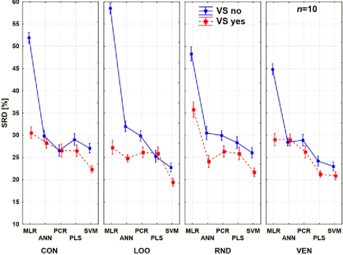
Figure 4. Results of factorial ANOVA with three factors. Blue continuous line means no variable selection (VS no), while the red dashed line corresponds to the variable selected models.
Normalized SRD values (%) are plotted on the y axis.
Figure 4 shows that with each cross-validation variant, MLR performed the worst, especially without variable selection. On the other hand, based on the predicted values, SVM is very promising (with and without variable selection). It seems that the importance of variable selection for SVM is less than for other methods. The shapes of the lines are quite similar to each other in the different cases. The plots were made with the use of the average values as the reference as well, and the results were very similar to Figure 4. This version can be found in Suppl. Mat. Fig. 1. In that case SRD values were lower, thus all-in-all the models were closer to the consensus. If we
pick another point of view in ANOVA analysis, we can see on Figure 5 the differences between the behaviors of the methods according to the cross-validation variants.
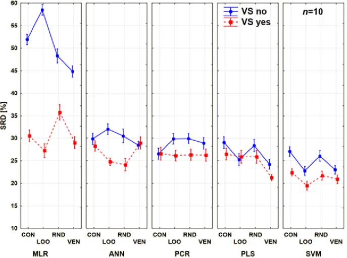
Figure 5. Results of factorial ANOVA with three factors. Blue continuous line means no variable selection (VS no), and the red dashed line corresponds to the variable selected models. Normalized SRD values (%) are plotted on the y axis.
It seemed that PCR was the most robust technique, because we can detect only minor changes between the use of different cross-validation variants (as compared to the other modeling methods), but on the other hand it rarely gave us the best model. This plot also reveals the huge differences in the case of MLR with and without variable selection, thus in this case the variable selection has a bigger importance than the validation types. From another point of view, the use of different validation variants is always case-dependent. It seems that every method has its own
“favorite” type, which can give us the most reliable results. However, we can conclude that the
contiguous block variant is never the best option. The results acquired with the use of the average as the reference show a very similar pattern with lower SRD values and can be found in Suppl.
Mat. Fig. 2.
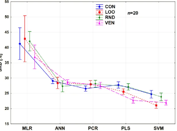
Factorial ANOVA was also performed with the use of modeling methods and CV variants as factors. In this case, variable selection was not a separation factor, the models with or without VS were used together. In Figure 6. one can understand the differences amongst the optimization opportunities, thus it can be a nice conclusion of Case study 1. In this figure we can see the decreasing magnitude of the SRD values between the different methods. SVM clearly gave the best results in all forms of cross-validation compared to the others, and MLR has much bigger errors than the other techniques. Thus, MLR is not recommended if we have a chance to apply more sophisticated methods.
Figure 6. Results of factorial ANOVA with two factors for Case study 1. Average SRD values (%) are plotted against the different methods. The cross-validation variants are plotted with different types of lines and shapes.
In each ANOVA analysis, the factors of cross-validation, methods and variable selection had always a statistically significant difference at the α = 0.05 value. Thus, proper optimization is always needed for each regression method we might choose.
Comparison based on SRD values for case study 2
In Case study 2 the same workflow was performed and the optimization parameters were tested with the same conditions. In this part, leave-one-out cross-validation was omitted from modeling with ANN due to the very long calculation time (over 24 hours). In this sense, this variant cannot be recommended for larger datasets. Based on the predicted values of internal and external validations, the models were compared with SRD and ANOVA methods. All the examined factors (CV, modeling methods and the use of variable selection) were significant at α = 0.05. Figure 7 shows the result of ANOVA with the use of the aforementioned factors.
Figure 7. Results of factorial ANOVA for Case study 2. Blue continuous line means no variable selection (VS no), and the red dashed line corresponds to the variable selected models. Normalized SRD values (%) are plotted on the y axis.
For Case study 2, there were bigger differences between the MLR and PCR models based on the use of variable selection. Again, SVM gave the best models for each type of CV variants. We can conclude that the contiguous block variant of CV was always the worst option and Venetian blinds were always among the best ones. (The same patterns can be observed with the use of the average as reference in SRD evaluations as well, see Supp. Mat. Fig. 3.)
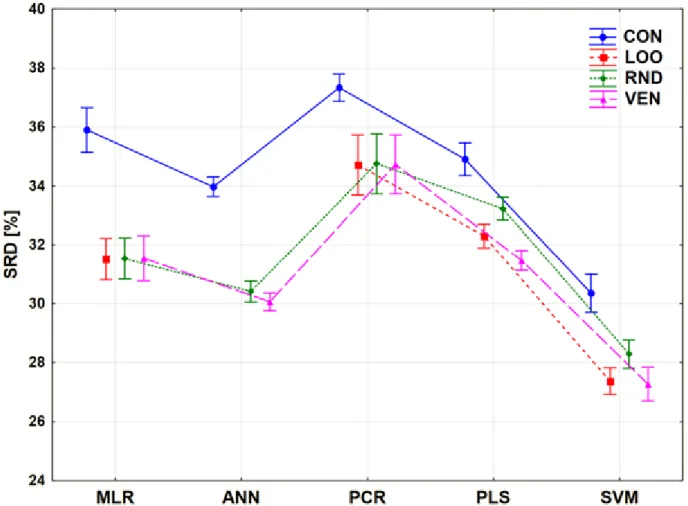
The comparison was also performed with only two factors: the CV variants and the modeling methods. The trends among the modeling methods and CV variants are clearly summarized in Figure 8.
Figure 8. Results of factorial ANOVA with two factors for Case study 2. Average SRD values (%) are plotted against the different methods. The cross-validation variants are plotted with different types of lines and shapes.
MLR and PCR are still not recommended for usual situations, even if PCR is a very robust technique in the sense of validation. On the other hand, PCR and MLR have the largest bias (largest SRD value), as compared to the other modeling methods. The most recommended one is SVM, but the use of the contiguous block CV variant is, again, highly discouraged. It is also clear how different results can be produced with the use of contiguous blocks compared to the other types.
If we compared the models to the average values instead of the experimental, the same patterns can be seen, which means that our findings revealed not just the best combinations but the most consistent ones as well. With the use of average we could decrease the systematic error, but on the other hand it gave a more compressed evaluation.
Conclusion
Based on the two case studies, the examined parameters had significant effects on model building.
In both studies support vector machines (SVM) performed the best and multiple linear regression (MLR) the worst. Although SVM was not as robust based on the performance parameters as partial least squares (PLS) regression or principal component regression (PCR), the sum of (absolute) raking difference (SRD) values obviously proved that even if it has quite bigger differences between calibration and validation, it can be a promising and well-optimized tool in regression model building tasks. The largest bias was reached with the contiguous blocks cross-validation (CV) variant and the MLR method. These two options are not recommended: neither alone, nor in combination. On the other hand, the use of variable selection is advisable in any case (and is an absolute must for MLR). We can conclude that the modeling techniques had a larger influence than CV variants in the evaluation of the models.
In summary, SRD provides a unique and unambiguous ranking of regression models, which helped to compare the different optimization protocols as well. Based on the two case studies and the use of predicted values, we could observe that the outcome of CV variants is data set dependent, still some major conclusions can be drawn: the contiguous blocks variant is an outdated form of CV, which can mislead our validation; the other three types are roughly equivalent on average, while the best choice from them is method dependent.
Acknowledgement
This work was supported by the National Research, Development and Innovation Office of Hungary (NKFIH, grants K 119269 and KH_17 125608).
Disclosure statement
No potential conflict of interest was reported by the authors.
ORCID
A. Rácz http://orcid.org/0000-0001-8271-9841 D. Bajusz http://orcid.org/0000-0003-4277-9481 K. Héberger http://orcid.org/0000-0003-0965-939X
References
[1] C. Hansch and T. Fujita, p-σ-π Analysis. A Method for the Correlation of Biological Activity and Chemical Structure, J. Am. Chem. Soc. 86 (1964), pp. 1616–1626.
[2] C. Hansch, P.P. Maloney, T. Fujita and R.M. Muir, Correlation of Biological Activity of Phenoxyacetic Acids with Hammett Substituent Constants and Partition Coefficients, Nature 194 (1962), pp. 178–180.
[3] L.P. Hammett, The Effect of Structure upon the Reactions of Organic Compounds. Benzene Derivatives, J. Am. Chem. Soc. 59 (1937), pp. 96–103.
[4] H. Kubinyi, QSAR : Hansch analysis and related approaches, VCH, 1993.
[5] A. Cherkasov, E.N. Muratov, D. Fourches, A. Varnek, I.I. Baskin, M. Cronin, J. Dearden, P. Gramatica, Y.C. Martin, R. Todeschini, V. Consonni, V.E. Kuz’min, R. Cramer, R.
Benigni, C. Yang, J. Rathman, L. Terfloth, J. Gasteiger, A. Richard and A. Tropsha, QSAR modeling: where have you been? Where are you going to? J. Med. Chem. 57 (2014), pp.
4977–5010.
[6] D. Bajusz, A. Rácz and K. Héberger, Chemical Data Formats, Fingerprints, and Other Molecular Descriptions for Database Analysis and Searching, in Comprehensive Medicinal Chemistry III, S. Chackalamannil, D.P. Rotella and S.E. Ward, eds., Elsevier, Oxford, 2017, pp. 329–378.
[7] T. Hastie, R. Tibshirani and J.H. Friedman, Cross-Validation, in The Elements of Statistical Learning: Data Mining, Inference, and Prediction, Springer, New York, 2009, pp. 241–249.
[8] R.D. Cramer, D.E. Patterson and J.D. Bunce, Comparative molecular field analysis (CoMFA). 1. Effect of shape on binding of steroids to carrier proteins, J. Am. Chem. Soc.
110 (1988), pp. 5959–5967.
[9] J. Verma, V. Khedkar and E. Coutinho, 3D-QSAR in Drug Design - A Review, Curr. Top.
Med. Chem. 10 (2010), pp. 95–115.
[10] S. Alam and F. Khan, 3D-QSAR studies on Maslinic acid analogs for Anticancer activity against Breast Cancer cell line MCF-7, Sci. Rep. 7 (2017), pp. 6019.
[11] A.M. Doweyko, 3D-QSAR illusions, J. Comput. Aided. Mol. Des. 18 (2004), pp. 587–596.
[12] K.H. Esbensen and P. Geladi, Principles of Proper Validation: use and abuse of re-sampling for validation, J. Chemom. 24 (2010), pp. 168–187.
[13] P. Gramatica, Principles of QSAR models validation: internal and external, QSAR Comb.
Sci. 26 (2007), pp. 694–701.
[14] D.M. Hawkins, S.C. Basak and D. Mills, Assessing model fit by cross-validation., J. Chem.
Inf. Comput. Sci. 43 (2003), pp. 579–86.
[15] D.M. Hawkins, The problem of overfitting., J. Chem. Inf. Comput. Sci. 44 (2004), pp. 1–12.
[16] A. Rácz, D. Bajusz and K. Héberger, Consistency of QSAR models: Correct split of training and test sets, ranking of models and performance parameters, SAR QSAR Environ. Res. 26 (2015), pp. 683–700.
[17] K. Héberger, A. Rácz and D. Bajusz, Which Performance Parameters Are Best Suited to Assess the Predictive Ability of Models? in Advances in QSAR Modeling, K. Roy, ed., Springer, 2017, pp. 89–104.
[18] J.C. Dearden, M.T.D. Cronin and K.L.E. Kaiser, How not to develop a quantitative structure–activity or structure–property relationship (QSAR/QSPR), SAR QSAR Environ.
Res. 20 (2009), pp. 241–266.
[19] T. Hanser, C. Barber, J.F. Marchaland and S. Werner, Applicability domain: towards a more formal definition., SAR QSAR Environ. Res. 27 (2016), pp. 893–909.
[20] P. Gramatica and A. Sangion, A Historical Excursus on the Statistical Validation Parameters for QSAR Models: A Clarification Concerning Metrics and Terminology, J. Chem. Inf.
Model. 56 (2016), pp. 1127–1131.
[21] O. Farkas, K. Héberger, Comparison of Ridge Regression, Partial Least Squares, Pair-wise Correlation, Forward- and Best Subset Selection Methods for Prediction of Retention Indices for Aliphatic Alcohols, J. Chem. Inf. Model., 45 (2005), 339 -346,
[22] J. P. Doucet, E. Papa, A. Doucet-Panaye & J. Devillers, QSAR models for predicting the toxicity of piperidine derivatives against Aedes aegypti, SAR QSAR Environ. Res. 28 (2017), pp. 451-470.
[23] J. A. Castillo-Garit, G. M. Casañola-Martin, S. J. Barigye, H. Pham-The, F. Torrens & A.
Torreblanca, Machine learning-based models to predict modes of toxic action of phenols to Tetrahymena pyriformis, SAR QSAR Environ. Res. 28 (2017), pp. 735-747.
[24] S. Bitam, M. Hamadache & S. Hanini, QSAR model for prediction of the therapeutic potency of N-benzylpiperidine derivatives as AChE inhibitors, SAR QSAR Environ. Res. 28 (2017), pp. 471-489.
[25] D. Qu, A. Yan & J. S. Zhang, SAR and QSAR study on the bioactivities of human epidermal growth factor receptor-2 (HER2) inhibitors, SAR QSAR Environ Res. 28 (2017), pp. 111- 112
[26] K. Héberger, S. Kolarević, M. Kračun-Kolarević, K. Sunjog, Z. Gačić, Z. Kljajić, M. Mitrić and B. Vuković-Gačić, Evaluation of single-cell gel electrophoresis data: combination of variance analysis with sum of ranking differences., Mutat. Res. - Genet. Toxicol. Environ.
Mutagen. 771 (2014), pp. 15–22.
[27] C. Bertinetto, C. Duce, R. Solaro and K. Héberger, Modeling of the Acute Toxicity of Benzene Derivatives by Complementary QSAR Methods, MATCH-COMMUNICATIONS Math. Comput. Chem. 70 (2013), pp. 1005–1021.
[28] M. Cassotti, D. Ballabio, V. Consonni, A. Mauri, I. V Tetko and R. Todeschini, Prediction of acute aquatic toxicity toward Daphnia magna by using the GA-kNN method., Altern. Lab.
Anim. 42 (2014), pp. 31–41.
[29] Schrödinger Release 2017-4: QikProp, Schrödinger, LLC, New York, NY, 2017. . [30] RDKit: Open-Source Cheminformatics Software; available at http://rdkit.org/.
[31] PLS Toolbox, Eigenvector Research Inc.; available at:
http://www.eigenvector.com/index.htm.
[32] A. Rácz, M. Fodor and K. Héberger, Development and comparison of regression models for the determination of quality parameters in margarine spread samples using NIR spectroscopy, Anal. Methods 10 (2018), pp. 3089–3099.
[33] K. Héberger, Sum of ranking differences compares methods or models fairly, TrAC Trends Anal. Chem. 29 (2010), pp. 101–109.
[34] K. Kollár-Hunek and K. Héberger, Method and model comparison by sum of ranking differences in cases of repeated observations (ties), Chemom. Intell. Lab. Syst. 127 (2013), pp. 139–146.
[35] D. Bajusz, A. Rácz and K. Héberger, Why is Tanimoto index an appropriate choice for fingerprint-based similarity calculations?, J. Cheminform. 7 (2015), pp. 20.
[36] G. Tóth, Z. Bodai and K. Héberger, Estimation of influential points in any data set from coefficient of determination and its leave-one-out cross-validated counterpart., J. Comput.
Aided. Mol. Des. 27 (2013), pp. 837–44.