Mathematical Biology

https://doi.org/10.1007/s00285-019-01424-6

Mathematical Biology

Delay in booster schedule as a control parameter in vaccination dynamics

Zhen Wang¹·Gergely Röst^2,3 ·Seyed M. Moghadas¹

Received: 23 June 2018 / Revised: 16 August 2019 / Published online: 7 September 2019

© The Author(s) 2019

Abstract

The use of multiple vaccine doses has proven to be essential in providing high levels of protection against a number of vaccine-preventable diseases at the individual level.

However, the effectiveness of vaccination at the population level depends on several key factors, including the dose-dependent protection efficacy of vaccine, coverage of primary and booster doses, and in particular, the timing of a booster dose. For vaccines that provide transient protection, the optimal scheduling of a booster dose remains an important component of immunization programs and could significantly affect the long-term disease dynamics. In this study, we developed a vaccination model as a sys- tem of delay differential equations to investigate the effect of booster schedule using a control parameter represented by a fixed time-delay. By exploring the stability anal- ysis of the model based on its reproduction number, we show the disease persistence in scenarios where the booster dose is sub-optimally scheduled. The findings indicate that, depending on the protection efficacy of primary vaccine series and the coverage of booster vaccination, the time-delay in a booster schedule can be a determining fac- tor in disease persistence or elimination. We present model results with simulations for a vaccine-preventable bacterial disease,Heamophilus influenzaeserotype b, using parameter estimates from the previous literature. Our study highlights the importance of timelines for multiple-dose vaccination in order to enhance the population-wide benefits of herd immunity.

Keywords Vaccination·Booster schedule·Delay equations·Reproduction number·Persistence

GR acknowledges the support of NKFIH Grant FK124016 and the Ministry of Human Capacities, Hungary Grant 20391-3/2018/FEKUSTRAT. SM acknowledges the support from the Natural Sciences and Engineering Research Council of Canada (NSERC) Discovery Grant, and the Mathematics of Information Technology and Complex Systems (MITACS), Canada.

B

Extended author information available on the last page of the article

Mathematics Subject Classification Primary 92D30; Secondary 93C23·34K05· 37M05

1 Introduction

Vaccination remains the most effective intervention measure in preventing many infec- tious diseases (Ehreth2003). Conferring high levels of protection against a number of vaccine-preventable diseases requires more than one dose of vaccine that may be offered at different ages according to specific schedules set by vaccination programs (Jackson et al.2012; Riolo et al.2013; Riolo and Rohani2015). For instance, vaccine schedules againstHaemophilus influenzaeserotype b (Hib) recommended for infants includes either 3 primary doses without a booster, or 2 to 3 primary doses plus a booster given at least 6 months after completing the primary series (World Health Organization et al.2016). However, even in the presence of booster doses, resurgence and outbreaks of some vaccine-preventable diseases still occur, notwithstanding substantial levels of routine primary vaccine series (Jackson et al.2012; Riolo et al.2013; Riolo and Rohani 2015). Reduced effectiveness of vaccination has been explicated for the occurrence of such outbreaks due to factors associated with incomplete protection efficacy of primary vaccine series, inadequate coverage of booster doses, waning immunity over time, and the duration of vaccine-induced protection that may be significantly shorter than the average lifetime of the population (Alexander et al.2006; Riolo and Rohani2015).

While the importance of age-at-vaccination and booster doses has been docu- mented, the optimal vaccine schedules remains unclear for several vaccine-preventable diseases and scheduling is mainly determined based on epidemiological context in individual settings (Low et al.2013; Jackson et al.2013; Riolo and Rohani2015). The diversity of booster dose schedules observed in immunization programs worldwide could have a significant impact on disease elimination, since the scheduling may also affect the uptake rates of booster vaccination (Fitzwater et al.2010). This poses a particular challenge for public health immunization programs in the context of defer- ral and subsequent refusal of booster doses that diminish the herd immunity (Omer et al.2009; Dubé et al.2013; Briere et al.2014), and could lead to disease resurgence.

Identification of the optimal booster schedule is therefore an important component of vaccination policies.

Despite the importance of dosing interval between primary and booster vaccina- tion, a theoretical framework to investigate the impact of such interval and varying vaccination schedules on disease dynamics in the population is currently lacking. In this study, we aimed to establish this framework by developing a vaccination model, represented by a system of delay differential equations that describe the dynamics of disease transmission. Using this system, we evaluated the effect of delay in booster dose after primary vaccination on the long-term disease prevalence. We incorporated a number of key parameters into the model including the protection efficacy of primary vaccination, duration of vaccine-induced protection, and the coverages of primary and booster vaccination. We considered the delay as a control parameter, and analyzed the transient and steady-state behaviours of the system, in addition to determining the effect of time interval between primary and booster doses on disease elimination and

persistence. We show, by means of simulations, that the threshold of disease control depends critically on the parameter of delay in booster dose for a given protection efficacy of primary vaccination.

To study the dynamics of our vaccination model, we first propose a basic framework without vaccination, derive the basic reproduction number (R0), and prove a threshold result for disease elimination in terms ofR0. We then construct the general model by incorporating primary and booster vaccination into the basic framework, and analyze its behaviour. Stability of the disease-free equilibrium is investigated, and represented in terms of the control reproduction number (Rc). WhenRc >1, we show the uni- form persistence, indicating that the disease elimination is infeasible. Finally, we use parameter values estimated for a bacterial disease,Heamophilus influenzaeserotype b (Hib), and perform simulations to illustrate the model results by varying time interval between primary and booster doses, represented by the delay parameter.

2 The basic framework

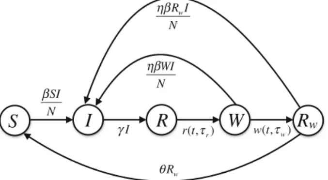
To develop the basic framework, we divided a population of constant sizeNinto several compartments to represent the epidemiological statuses of individuals as susceptible (S), infectious (I), recovered and fully protected (R), and partially protected (W, and R_w). The distinction between the two classesWandR_wis based on the consideration that partial protection following natural infection may last for a certain period of time (on average) before declining towards negligible levels. We assumed a fixed duration of full protection following recovery from infection. Once this period has elapsed, individuals will have only partial protection, and may become infected at a reduced rate compared with fully susceptible individuals. The duration of partial protection is divided into a period of fixed length (for those in theW class), followed by an exponentially distributed period of waning immunity (for those in theR_wclass) leading to full susceptibility. Due to the fixed periods of full and partial protection, the dynamics of disease transmission can be expressed by the following set of equations:

S(t)=μN−βS I

N −μS+θR_w, I(t)= βS I

N +ηβW I

N +ηβR_wI

N −γI −μI, R(t)=

_τr

0

r(t,a)da, W(t)=

_τw

0 w(t,a)da, R_w(t)=w(t, τw)−ηβR_wI

N −μR_w−θR_w, (1)

whereβis the baseline transmission rate;γ is the recovery rate of infectious individ- uals,ηis the reduction of susceptibility to infection due to partial protection,μis the natural death rate (assumed to be the same as the birth rate),τr represents the fixed duration of full protection,τwrepresents the fixed duration of partial protection; and

R_wI N

WI SI N

N

I r(t, _r) w(t, _w)

S I R W R

R_w

Fig. 1 Schematic diagram for the basic structure of the model in the absence of vaccination

θis the rate of loss of immunity in partially protected individuals in the R_wclass. A schematic diagram of the transitions between different classes of individuals in this basic framework is represented in Fig.1.

Leta, referred to as ‘age’, be the time elapsed since individuals enter each class.

Thus,r(t,a)andw(t,a)represent the density, with respect to agea at timet, of recovered individuals having full protection, and those having partial protection during the fixed period before moving to the exponentially distributed period, respectively.

Using the above notation, we have the following equations:

∂

∂t + ∂

∂a

r(t,a)= −μr(t,a), r(t,0)=γI(t), ∂

∂t + ∂

∂a

w(t,a)= −μw(t,a)−ηβI(t)

N w(t,a), w(t,0)=r(t, τr).

(2)

Solving along the characteristics gives:

r(t, τr)=r(t−τr,0)e^−μτr =γI(t−τr)e^−μτr,

w(t, τw)=w(t−τw,0)e

−μτw−ηβˆ

_t

t−τw

I(u)du

=r(t−τ_w, τr)e^{−μτw−η}

βˆ

_t

t−τw

I(u)du

=γI(t−τr −τw)e

−μ(τr+τw)−ηβˆ

_t

t−τw

I(u)du ,

(3)

where, for simplicity we used the notationβˆ =β/N. Note that system (1) includes integral and differential equations. By differentiating the RandW equations in (1) with respect tot, we obtain the following model, which together with (3), constitutes a closed system of delay differential equations:

S(t)=μN− ˆβS I −μS+θR_w,

I(t)= ˆβS I +ηβˆW I+ηβˆR_wI−γI−μI, R(t)=γI−μR−r(t, τr),

W(t)=r(t, τr)−ηβˆW I−μW −w(t, τ_w), R_w(t)=w(t, τ_w)−ηβˆR_wI−μR_w−θR_w.

(4)

One can easily check that the populationN(t)=S(t)+I(t)+R(t)+W(t)+R_w(t) is indeed constant.

Letτ =τr+τ_w, and denote byCthe Banach spaceC([−τ,0],R⁵)of continuous functions mapping the interval[−τ,0]intoR⁵equipped with the norm:

φ = sup

θ∈[−τ,0]|φ(θ)|,

whereφ∈Cand| · |is a norm inR⁵. For a continuous functionu: [−τ, σ_φ)→R⁵ withσ_φ>0, we defineut ∈Cfor eacht≥0 byut(θ)=u(t+θ), for allθ∈ [−τ,0].

We choose the initial conditions for system (4) from the setΩ ⊆C, defined by:

Ω=

φ∈C :φi(s)≥0, s∈ [−τ,0], 1≤i≤5, φ3(0)=

_τr

0

γe^−μaφ2(−a)da, φ4(0)=

_τw

0

γe^{−μ(τr+a)−ηβˆ}

0

−aφ2(u)duφ2(−τr−a)da .

(5)

The following result shows that system (4) is well-posed inΩ, and the solution semiflow admits a global attractor onΩ.

Theorem 2.1 For anyφ ∈Ω, system(4)has a unique non-negative solution u(t, φ) satisfying u0=φand ut ∈Ωfor all t>0, and the solution semiflowΦ(t)=ut(·): Ω → Ω has a compact global attractor. Moreover, the solutions of system(4)with initial conditions inΩsatisfy the integro-differential equations system(1).

Proof We start with the last assertion. From the third equation of (4), we have:

e^μt(R(t)+μR(t))=γe^μt(I(t)−I(t−τr)e^−μτr).

Integrating both sides yields:

e^μtR(t)−R(0)=γ t

0

e^μsI(s)ds− _t

0

e^μsI(s−τr)e^−μτrds

=γ _t

0

e^μsI(s)ds− _t−τr

−τr

e^μsI(s)ds

=γ t

t−τr

e^μsI(s)ds−γ 0

−τr

e^μsI(s)ds.

Therefore, withR(0)=γ0

−τr e^μsI(s)ds =γ_τr

0 e^−μaI(−a)da, we have:

R(t)=γ _t

t−τr

e^μsI(s)ds=γ _τr

0

e^−μaI(t−a)da= _τr

0

r(t,a)da. (6)

Similarly, by integrating e^{μt+ηβˆ0tI(u)du}

W(t)+μW(t)+ηβˆI(t)W(t) ,

and using the initial conditionW(0)=_τw

0 γe^{−(τr+a)−ηβˆ}

0

−aI(u)du

I(−τr−a)da, the differential equationW(t)in (4) gives:

W(t)=γ _τw

0

γI(t−τr−a)e^{−μ(τr+a)−ηβˆ} _t

t−a

I(u)du da=

_τw

0

w(t,a)da. (7)

For a givenφ∈C, we define

G(φ):=(G1(φ),G2(φ),G3(φ),G4(φ),G5(φ)), with

G1(φ)=μN− ˆβφ1(0)φ2(0)−μφ1(0)+θφ5(0),

G2(φ)= ˆβφ1(0)φ2(0)+ηβφˆ 2(0)φ4(0)+ηβφˆ 2(0)φ5(0)−(γ +μ)φ2(0), G3(φ)=γ φ2(0)−μφ3(0)−γ φ2(−τr)e^−μτr,

G4(φ)=γ φ2(−τr)e^−μτr −ηβφˆ 2(0)φ4(0)−μφ4(0)

−γ φ2(−τr−τ_w)e^{−μ(τr+τw)−ηβˆtt−τwφ2(s)ds},

G5(φ)=γ φ2(−τr−τ_w)e^{−μ(τr+τw)−ηβˆtt−τwφ2(s)ds}−ηβφˆ 2(0)φ5(0)

−(μ+θ)φ5(0).

Thus, system (4) can be written asu(t)=G(ut). We show thatG(φ)is Lipschitzian inφwithin each compact set inC, that is for allM >0 there is aK >0 such that for all φ, ψ∈Cwithφ ≤Mandψ ≤M, the inequality|G(φ)−G(ψ)| ≤Kφ−ψ holds. We note that there are terms of linear, quadratic and exponential types inG.

Quadratic terms are all Lipschitzian, and one can see that:

|φ1(0)φ2(0)−ψ1(0)ψ2(0)| ≤ |φ1(0)φ2(0)−φ1(0)ψ2(0)|

+|φ1(0)ψ2(0)−ψ1(0)ψ2(0)|

≤2Mφ−ψ.

The Lipschitzian property for the most involved term can also be seen from:

|φ2(−τ)e^{−ηβˆtt−τwφ2(s)ds}−ψ2(−τ)e^{−ηβˆtt−τwψ2(s)ds}|

≤ |φ2(−τ)e^{−ηβˆtt−τwφ2(s)ds}−φ2(−τ)e^{−ηβˆtt−τwψ2(s)ds}| +|φ2(−τ)e^−ηβˆ

t

t−τwψ2(s)ds−ψ2(−τ)e^−ηβˆ

t

t−τwψ2(s)ds|

≤ Me^{ηβτˆ wM}ηβτˆ wφ−ψ +e^{ηβτˆ wM}φ−ψ,

where we used the mean value theoreme^x−e^y =e^ξ(x−y). Hence, there is a unique solution of the system through(0, φ)on its maximal interval of existence[0, σφ). We note from (4) that any solution satisfies:

I(t)=I(0)e^{0tβˆS(u)+ηβˆW(u)+ηβˆRw(u)−γ−μdu}, (8) and hence ifI(0)≥ 0, thenI(t)≥ 0 for allt ∈ (0, σ_φ). From (6) and (7), we find thatRandWare non-negative. Then the non-negativity ofSandR_wfollows from the inequalities

S(t)≥μN− ˆβS I−μS, and

R_w(t)≥ −ηβˆR_wI−μR_w−θR_w.

The non-negativity and relations (6) and (7) ensure thatΩis forward invariant. Since the total population is constant, it follows thatS(t)andI(t)are bounded byN and the solutions exist globally. Therefore, the solution semiflowΦ(t)=ut(·):Ω →Ω is point dissipative. By Theorem 3.6.1 in Hale (1977),Φ(t)is compact for anyt> τ. Thus, from Theorem 3.4.8 in Hale (1988), it follows thatΦ(t)has a compact global attractor inΩ.

2.1 Basic reproduction number

The basic reproduction number (R0) is the average number of new infected individ- uals generated by a single infected individual introduced into an entirely susceptible population, during the course of infection. According to the theory of epidemics, we expect that the disease will vanish ifR0 <1, while it will persist in the population ifR0>1. New infections occur only in theSclass with the rateβˆI. In a fully sus- ceptible population,S/N ≈1 and the average length of infection is(μ+γ )⁻¹, and therefore we define the basic reproduction number asR0=β/(γ +μ). We proceed by presenting the threshold dynamics for system (4), which determines whether the disease dies out or persists.

2.2 Threshold dynamics

It is clear that system (4) has a unique disease-free equilibriumE0=(N,0,0,0,0). We first show that E0 is globally asymptotically stable when R0 < 1. Then we establish the uniform persistence of the disease whenR0 > 1 using techniques of persistence theory (Smith and Thieme2011).

Theorem 2.2 IfR0<1, then the disease-free equilibrium E0of system(4)is globally asymptotically stable inΩ.

Proof Linearizing system (4) atE0, we obtain the following system:

u(t)=A1u(t)+A2u(t−τr)+A3u(t−τr −τw), (9) whereu(t)=(S(t),I(t),R(t),W(t),R_w(t))^T, and

A1=

⎛

⎜⎜

⎜⎜

⎝

−μ −β 0 0 θ

0 β−γ −μ 0 0 0

0 γ −μ 0 0

0 0 0 −μ 0

0 0 0 0 −(μ+θ)

⎞

⎟⎟

⎟⎟

⎠,

A2=(A2)i j, 1≤i,j ≤5, with(A2)32 = −γe^−μτr,(A2)42=γe^−μτr and all other components are zero; A3 = (A3)i j, 1 ≤ i,j ≤ 5, with(A3)42 = −γe^{−μ(τr+τw)}, (A3)52=γe^{−μ(τr+τw)}and all other components are zero. The characteristic equation of system (9) has the form:

det(λI−A1−e^−τrλA2−e^{−(τr+τw)λ}A3)=0,

which gives(λ+μ)³(λ+μ+θ)(λ−β +γ +μ) = 0. SinceR0 < 1, we have β−(γ +μ) <0, which implies that E0is asymptotically stable.

Now we prove thatE0is globally attractive inΩ. We consider the following inequal- ity:

I(t)≤ ˆβ(S+W +R_w)I−(γ +μ)I ≤(R0−1)(γ+μ)I.

Thus,I(t) ≤ I(0)e^{(R0−1)(γ+μ)t}, and hence I(t)→ 0 ast → ∞. From (6) and (7), we find thatR(t)andW(t)are also converging to zero. For any > 0, and a sufficiently larget >0, we havew(t, τw) < , and the following inequality holds:

R_w (t)≤−(μ+θ)R_w. This means that lim sup

t→∞ R_w(t)≤

μ+θ, and thereforeR_w→0 ast → ∞. Since the total population is constant, we obtain thatS(t)→ Nast → ∞. Thus, lim

t→∞u(t, φ)= (N,0,0,0,0), and we conclude thatE0is globally asymptotically stable.

We now prove the persistence of disease forR0>1. Considering the semiflowΦ onΩ, we define the persistence function by:

P:Ω→R₊, P(φ)=φ2(0).

Let

Ω₊:= {φ∈Ω|P(φ) >0},

Ω0:= {φ∈Ω|P(φ)=0} =Ω\Ω+,

whereΩ0is called the extinction space corresponding toP(that is the collection of states where the disease is not present). From the relation (8), it follows that the sets Ω0 andΩ₊ are forward invariant under the semiflowΦ. We now introduce some terminology from persistence theory (Smith and Thieme2011, Chapters 3.1 and 8.3).

Definition 2.3 LetXbe a nonempty set andP: X→R₊.

1. A semiflowΦ :R₊×X → X is called uniformly weaklyP-persistent, if there exists some >0 such that

lim sup

t→∞ P(Φ(t,x)) > ∀x∈ X, P(x) >0.

2. A semiflow Φ is called uniformly (strongly) P-persistent, if there exists some >0 such that

lim inf

t→∞ P(Φ(t,x)) > ∀x ∈X, P(x) >0.

3. A setM ⊆Xis called weaklyP-repelling if there is nox∈ Xsuch thatP(x) >0 andΦ(t,x)→M ast → ∞.

Theorem 2.4 IfR0>1, then the semiflowΦ is uniformly P-persistent, i.e., there is aδ >0such that for any solutionlim inft→∞I(t)≥δ.

Proof First we show thatE0is weaklyP-repelling. Suppose that there existsψ0∈Ω such thatP(ψ0) >0 with

tlim→∞Φ(t, ψ0)=E0. (10)

For such a solution,I(0) >0 and limt→∞I(t)=0. Let >0 small so thatR0(1−

N) >1. Thus, for sufficiently larget we haveΦ(t, ψ0)−E0< , and

I≥ ˆβS I−(γ +μ)I ≥ β(N−)

N I−(γ +μ)I

=

R0(1−

N)−1 (γ +μ)I >0,

Table 1 Description of vaccine-related individual classes in the vaccination model

Variable Description

Vs Newborns who will receive primary vaccine inτsperiod of time following birth

Vp Primary vaccinated individuals who may receive booster dose

V_d Partially protected individuals who will not receive booster dose

V_w Primary vaccinated individuals in whom vaccine-induced protection wanes over

Vb Individuals who have received booster vaccination and are currently fully protected

which contradicts the convergence of I to zero. Hence, E0 is weakly P-repelling.

Notice that whenever I(t) ≡ 0, from (6) and (7) we have R(t) ≡ 0 ,W(t) ≡ 0, andw(t, τw) ≡ 0, and consequently R_w → 0 and S → N ast → ∞. Therefore

∪φ∈Ω0ω(φ)= {E0}, and one can see from Theorem 8.17 in Smith and Thieme (2011) thatΦ is uniformly weakly P-persistent. SinceΦhas a compact global attractor on Ω, we can apply Theorem 4.5 in Smith and Thieme (2011) to conclude thatΦ is uniformlyP-persistent.

Theorems2.2and2.4indicate that the disease dynamics are completely determined by the basic reproduction number R0. In the following, we extend our model by introducing the primary and booster vaccination, and analyze the persistence dynamics of the resulting system.

3 The general vaccination model

The vaccination model includes additional classes of individuals who are vaccinated with primary series; partially protected following primary vaccination; and fully pro- tected following booster vaccination (See Table1). A schematic diagram for timelines of primary and booster vaccination with delays is represented in Fig.2. We assume that a fractionpof newborns will receive primary vaccine series in the firstτs period of their life. The remaining fraction of newborns will be recruited to the susceptible class and can therefore become infected through contacts with infectious individu- als. The primary vaccination is assumed to provide partial protection for a certain period of time during which infection can occur with a lower rate compared with fully susceptible individuals. We also assume that partial protection induced by primary vaccine gradually wanes over time, and individuals who forgo booster vaccination will eventually become susceptible. Similar to the basic framework, we consider a fixed duration of partial protection after primary vaccination, followed by an expo- nentially distributed period of waning immunity leading to full susceptibility. Those who have received primary vaccination may also receive booster dose. We assume that, similar to recovery from infection, booster vaccination provides a fixed duration of full protection, followed by fixed and exponentially distributed durations of partial protection.

d p

s

birth loss of partial

protection

fully susceptible

booster vaccination

v_s(t,a) v_p(t,a) v_d(t,a) Vw

primary

vaccination b w

v_b(t,a) w(t,a)

loss of full protection

1 r

I

infection recovery

Fig. 2 Schematic diagram for timelines of primary and booster vaccination with delay, and durations of vaccine-induced and naturally acquired protection

In order to mathematically express the model, we letarepresent the age since the individuals enter each class, and definevs(t,a),vp(t,a), and vd(t,a)to represent the density, with respect to ageaat current timet, of primary vaccinated individuals, those who are partially protected as a result of primary vaccination and eligible to receive booster dose, and those who are partially protected by primary vaccination and will not receive booster dose, respectively. Letτp(0 ≤ τp ≤ τw) represent the delay in receiving booster vaccination within the fixed period of partial protection following primary vaccination. For those who will not receive the booster, we denote byτdthe remaining period of time within the fixed duration of partial protection, i.e., τp+τd =τ_w. Description of all model parameters are provided in Table2.

With the above notation, the model can be expressed by the following system of integro-differential equations:

S(t)=(1−p)μN− ˆβS I −μS+θV_w, Vs(t)=

_τs

0

vs(t,a)da, Vp(t)=

_τp

0

vp(t,a)da, Vd(t)=

_τd

0 vd(t,a)da,

V_w(t)=vd(t, τd)−ηβˆV_wI−(μ+θ)V_w+w(t, τ_w), Vb(t)=

_τb

0 vb(t,a)da, W(t)=

_τw

0

w(t,a)da,

I(t)= ˆβI[S+Vs+η(Vp+Vd+V_w+W)] −γI−μI,

Table 2 Description of the model parameters and their associated values (ranges) extracted from the pub- lished literature

Parameter Description Value (range)

R0 Basic reproduction number 1.2 (1.1–1.4)

μ Birth and natural death rate 1/70 per year

γ Recovery rate of infection 7.3 per year

β=R0(γ+μ) baseline transmission rate of infection 8.777 per year

p Coverage of primary vaccination 0.9 (0–1)

ρ Coverage of booster vaccination Variable (0–1)

η Reduced susceptibility during partial protection Variable (0–1)

τs Age at primary vaccination 6 months

τp Delay in booster vaccination Variable (0–4)

years

τw Fixed period of partial protection 4 years

τb Fixed period of full protection following booster 6 years τr Fixed period of full protection following recovery 4 years

θ Rate of loss of partial protection 0.1667 per year

R(t)= _τr

0

r(t,a)da, (11)

with population densities expressed by:

∂

∂t + ∂

∂a

vs(t,a)= −μvs(t,a)− ˆβI(t)vs(t,a),

vs(t,0)=pμN, (12)

∂

∂t + ∂

∂a

vp(t,a)= −μvp(t,a)−ηβˆI(t)vp(t,a),

vp(t,0)=vs(t, τs), (13) ∂

∂t + ∂

∂a

vd(t,a)= −μvd(t,a)−ηβˆI(t)vd(t,a),

vd(t,0)=(1−ρ)vp(t, τp), (14) ∂

∂t + ∂

∂a

vb(t,a)= −μvb(t,a),

vb(t,0)=ρvp(t, τp), (15)

∂

∂t + ∂

∂a

r(t,a)= −μr(t,a),

r(t,0)=γI(t), (16)

∂

∂t + ∂

∂a

w(t,a)= −μw(t,a)−ηβˆI(t)w(t,a),

w(t,0)=vb(t, τb)+r(t, τr). (17) In this model, we considered a single classV_w for partially protected individuals with exponentially distributed duration of protection, regardless of whether the immu- nity was conferred by vaccination or natural infection. Thus, the R_w class from the basic framework is included in theV_w class in the vaccination model. Solving along the characteristics gives:

vs(t, τs)=vs(t−τs,0)e^{−μτs− ˆβ} _t

t−τs

I(u)du

=pμN e

−μτs− ˆβ

_t

t−τs

I(u)du

,

vp(t, τp)=vp(t−τp,0)e

−μτp−ηβˆ

t t−τp

I(u)du

,

vd(t, τd)=vd(t−τd,0)e^{−μτd−ηβˆ} _t

t−τd

I(u)du

,

vb(t, τb)=vb(t−τb,0)e^−μτb =ρvp(t−τb, τp)e^−μτb, r(t, τr)=r(t−τr,0)e^−μτr =γI(t−τr)e^−μτr, w(t, τ_w)=w(t−τ_w,0)e^{−μτw−ηβˆ}

_t

t−τw

I(u)du .

(18)

Differentiating the integral equationsVs,Vp,Vd,Vb,W andRin (11) and substi- tuting the density functions, we obtain the following system of differential equations with delays:

S(t)=(1−p)μN− ˆβS I −μS+θV_w, V_s(t)= pμN

1−e^{−μτs− ˆβA} − ˆβVsI−μVs, V_p(t)= pμN

e^{−μτs− ˆβA}−e^{−μ(τs+τp)−ηβˆB− ˆβA(t−τp)} −ηβˆVpI−μVp, V_d(t)=(1−ρ)pμN e^{−μ(τs+τp)−ηβˆB− ˆβA(t−τp)}

−(1−ρ)pμN e^{−μ(τs+τp+τd)−ηβˆC− ˆβA(t−τw)}−ηβˆVdI−μVd, V_w(t)=(1−ρ)pμN e^{−μ(τs+τp+τd)−ηβˆC− ˆβA(t−τw)}−ηβˆV_wI−(μ+θ)Vw

+ρpμN e^{−μ(τs+τp+τb+τw)−ηβˆC−ηβˆB(t−τb−τw)− ˆβA(t−τp−τb−τw)} +γI(t−τr−τ_w)e^{−μτr−μτw−ηβˆC},

V_b(t)=ρpμN e^{−μ(τs+τp)−ηβˆB− ˆβA(t−τp)}−μVb

−ρpμN e^{−μ(τs+τp+τb)−ηβˆB(t−τb)− ˆβA(t−τp−τb)},

W(t)=ρpμN e^{−μ(τs+τp+τb)−ηβˆB(t−τb)− ˆβA(t−τp−τb)}−ηβˆW I −μW

−ρpμN e^{−μ(τs+τp+τb+τw)−ηβˆB(t−τb−τw)− ˆβA(t−τp−τb−τw)−ηβˆC}

−γ

I(t−τr−τ_w)e^{−μτw−ηβˆC}−I(t−τr)

e^−μτr, I(t)= ˆβ

S+Vs+η(Vp+Vd+V_w+W)

I −γI−μI,

R(t)=γI−γI(t−τr)e^−μτr −μR, (19) where

A(t)= _t

t−τs

I(u)du, B(t)= _t

t−τp

I(u)du, C(t)= _t

t−τw

I(u)du.

The total populationS(t)+Vs(t)+Vp(t)+Vd(t)+V_w(t)+Vb(t)+W(t)+I(t)+R(t)= N. Note that the equations ofVbandRare decoupled from the rest of the model.

In the following, we show that (19) is well-posed, and further define the disease- free equilibrium and the control reproduction number. Letτc=max{τs+τp+τb+ τ_w, τr +τ_w}. We choose the initial conditions for system (19) from the setX, which is defined by

X =

φ∈C([−τc,0],R⁹):φi(s)≥0, s∈ [−τc,0], 1≤i≤9, φ2(0)=

_τs

0

pμN e^{−μa− ˆβ}

0

−aφ8(s)dsda, φ3(0)=

_τp

0

pμN e^{−μ(τs+a)−ηβˆ}

0

−aφ8(s)ds− ˆβ₋a

−τs−aφ8(s)ds

da, φ4(0)=

_τd

0

(1−ρ)pμN e^{−μ(τs+τp+a)−ηβˆ−τp0 −aφ8(s)ds− ˆβ−τs−τp−−τpa−aφ8(s)ds}da, φ6(0)=

_τb

0

ρpμN e^{−μ(τs+τp+a)−ηβˆ−τp−a−aφ8(s)ds− ˆβ−τs−τp−−τpa−aφ8(s)ds}da, φ7(0)=

_τw

0 ρpμN e^{−μ(τs+τp+τb+a)−ηβˆ}

0

−aφ8(s)ds−ηβˆ−τb−a

−τp−τb−aφ8(s)ds

×e^{− ˆβ}

−τp−τb−a

−τs−τp−τb−aφ8(s)ds

+γ φ8(−τr−a)e^{−μ(τr+a)−ηβˆ}

0

−aφ8(s)ds

da, φ9(0)=

_τr

0

γe^−μaφ8(−a)da

. (20)

Theorem 3.1 For anyφ∈X, system (19) has a unique non-negative solution U(t, φ) satisfying U0 =φand Ut ∈ X, and the solution semiflowΦ(t)=Ut(·):X →X has a compact global attractor. Moreover, the solutions of system (19) with initial conditions inX satisfy the integro-differential equations system(11).

Proof The proof is similar to Theorem2.1.