A Comprehensive Study of the Parameters in theCreation and Comparison of Feature Vectors inDistributional Semantic Models

(1)

Full Terms & Conditions of access and use can be found at

https://www.tandfonline.com/action/journalInformation?journalCode=njql20

Journal of Quantitative Linguistics

ISSN: 0929-6174 (Print) 1744-5035 (Online) Journal homepage: https://www.tandfonline.com/loi/njql20

A Comprehensive Study of the Parameters in the Creation and Comparison of Feature Vectors in Distributional Semantic Models

András Dobó & János Csirik

To cite this article: András Dobó & János Csirik (2019): A Comprehensive Study of the

Parameters in the Creation and Comparison of Feature Vectors in Distributional Semantic Models, Journal of Quantitative Linguistics, DOI: 10.1080/09296174.2019.1570897

To link to this article: https://doi.org/10.1080/09296174.2019.1570897

Published online: 12 Mar 2019.

Submit your article to this journal

Article views: 364

View related articles

View Crossmark data

Citing articles: 1 View citing articles

(2)

A Comprehensive Study of the Parameters in the Creation and Comparison of Feature Vectors in Distributional Semantic Models

András Dobó and János Csirik

Institute of Informatics, University of Szeged, Szeged, Hungary

ABSTRACT

Measuring the semantic similarity and relatedness of words can play a vital role in many natural language processing tasks. Distributional semantic models computing these measures can have many diﬀerent parameters, such as diﬀerent weighting schemes, vector similarity measures, feature transformation functions and dimensionality reduction techniques. Despite their impor- tance there is no truly comprehensive study simultaneously evaluating the numerous parameters of such models, while also considering the interaction of these parameters with each other.

We would like to address this gap with our systematic study. Taking the necessary distributional information extracted from the chosen dataset as already granted, we evaluate all important aspects of the creation and comparison of feature vectors in distributional semantic models. Testing altogether 10 parameters simultaneously, we try toﬁnd the best combination of parameter settings, with a large number of settings examined in case of some of the parameters. Beside evaluating the conventionally used settings for the parameters, we also propose numerous novel variants, as well as novel combinations of parameter settings, some of which signiﬁcantly outperform the combinations of settings in general use, thus achieving state-of-the-art results.

1. Introduction

For many natural language processing (NLP) problems it is crucial to determine the semantic similarity or semantic relatedness of words, by which we mean how much the concepts denoted by the words are similar or related to each other, respectively. While relatedness takes a wide range of relations between concepts (including similarity) into account, similarity only considers how much the two concepts are truly alike. For example, the words‘postman’and‘mail’are highly related, as usually mails are delivered by postmen, but they are not similar, as they denote rather diﬀerent concepts.

CONTACTAndrás Dobó dobo@inf.u-szeged.hu

This article has been republished with minor changes. These changes do not impact the academic content of the article.

https://doi.org/10.1080/09296174.2019.1570897

This is an Open Access article distributed under the terms of the Creative Commons Attribution-NonCommercial- NoDerivatives License (http://creativecommons.org/licenses/by-nc-nd/4.0/), which permits non-commercial re-use, distribution, and reproduction in any medium, provided the original work is properly cited, and is not altered, transformed, or built upon in any way.

(3)

Most models calculate semantic similarity and relatedness using distributional data extracted from large corpora. These are collectively called distributional semantic models (DSMs) (Baroni, Dinu & Kruszewski,2014). In these models ﬁrst possible features are identiﬁed, usually in the form of context words, and then a weight is assigned to each word-feature pair, thus creating feature vectors for the words. The similarity or relatedness of words are then calculated by comparing their feature vectors. Although DSMs have many possible parameters, a truly comprehensive study of these parameters, also fully considering the dependencies between them, is still missing and would be needed, as also suggested by Levy, Goldberg, and Dagan (2015).

Most papers presenting DSMs focus on only one or two aspects of the problem, and take all the other parameters as granted with some standard setting, e.g. cosine as vector similarity measure and/or (positive) pointwise mutual information as weighting scheme out of convention. And even in case of the considered parameters, usually only a handful of possible settings are tested for. Further, there are also such parameters that are completely ignored by most studies (e.g. smoothing, vector normalization or minimum feature frequency). What’s more, as these parameters can influence each other greatly, evaluating them separately, one-by-one, would not even be sufficient, as that would not account for the interaction between them. There are a couple of studies that consider several parameters with multiple possible settings, such as Lapesa and Evert (2014) and Kiela and Clark (2014), but even these are far from being truly comprehensive, and do not fully test for the interaction between the different parameters. So, although an extensive analysis of the possible parameters and their combinations would be crucial (Levy et al.,2015), there has been no research to date that would have evaluated these truly comprehensively.

In this paper, we would like to address this gap.

DSMs have two distinct phases in general. In the first phase statistical information is extracted from raw data (i.e. a corpus). In the second phase, feature vectors are created from the extracted information for each word and these vectors are compared to each other to calculate the similarity or relatedness of words. We take the information extracted in thefirst phase as already granted, and present a systematic study simultaneously testing all important aspects of the creation and comparison of feature vectors in DSMs, also caring for the interaction between the different parameters.

We have chosen to only study the second phase of the DSMs, as the two phases are relatively distinct and independent from each other, and testing for every single possible combination of the parameter settings in the second phase is already unfeasible due to the vast number of combinations. Therefore we have omitted the examination of the ﬁrst phase completely, with one exception to this. DSMs have two major categories based on the type of theirﬁrst phase: count-vector-based (CVBM) and predictive

(4)

models (PM; also called word embeddings) (Baroni et al.,2014). In order to get a more complete view, we have done tests using information extracted from a corpus using both a CVBM and a PM. Our intuition is that there will be a single combination of parameter settings that achieves the best results in case of both CVBMs and PMs.

During our research we have identiﬁed 10 important parameters for the second phase of CVBMs, out of which only 4 are present in PMs due to the characteristics of such models. We have simultaneously evaluated each one with numerous settings toﬁnd the best combination of parameter settings (CPS) out of the billions of possible combinations. We also proposed numerous new settings in case of some parameters. Some of our novel CPSs considerably outperform the conventionally used combinations, achieving state-of-the-art results.

2. Background

Although even some early DSMs have experimented with trying multiple settings for one or more parameters, such as vector similarity measures, even in most state-of-the-art systems actually only one similarity measure (predominantly cosine similarity) was tested (e.g. Christopoulou, Briakou, Iosif, & Potamianos,2018; Salle, Idiart, & Villavicencio,2018; Speer, Chin,

& Havasi,2017; Vakulenko,2018). Further, most CVBMs only test for one weighting scheme (e.g. Levy et al., 2015; Salle et al., 2018), based on pointwise mutual information (PMI) (Church & Hanks, 1990) in almost all cases. Moreover, many of the other possible parameters, such as feature transformation or smoothing, have been completely neglected in the vast majority of studies.

Of course there are also a couple of studies that try to examine one or more of the parameters of DSMs in detail. Some of them focus solely on vector similarity measures (e.g. Weeds, 2003). On the other hand, others (e.g. Evert, 2005) evaluate diﬀerent weighting schemes extensively.

A handful of studies, such as Lapesa and Evert (2014) and Kiela and Clark (2014), also take other parameters into account, like feature transformation or dimensionality reduction. These more complex studies some- times also mix the parameters of the first phase of DSMs with those of the second phase of DSMs and thus also include parameters like source corpus, context type and context size. But even these studies usually neglect many other important aspects of the problem, do not account for the interaction between the different parameters sufficiently, and/or only test for a handful of different settings for each parameter. So evaluating all the possible parameters together and testing their possible combinations extensively would be crucial, but has not been addressed sufficiently yet.

(5)

3. Data and Evaluation Methods

A vast number of combinations of parameter settings (CPS) needed to be tested, therefore in case of the CVBMs we have chosen the relatively small British National Corpus (BNC; about 100 million words), from which the information was extracted by the bag-of-words method presented in Dobó

& Csirik (2013). Here the extracted raw counts were used, which will be referenced as Dobó and Csirik’s counts on the BNC (DcBnc). This method extracts information for nouns, verbs, adjectives and adverbs separately. We have used the original method presented in Dobó & Csirik (2013) to guess the part-of-speech of input words when creating their feature vectors.

For the PMs, corpus size was much less relevant with respect to the feasibility of our analysis, as much fewer parameters were tested, and the number of dimensions of the feature vectors was also small. We have decided on the Google News corpus (GNC) of around 100 billion words, from which feature vectors for words were created by Mikolov, Corrado, Chen, and Dean (2013).¹ These semantic vectors will be referenced as Mikolov et al.’s vectors (Mv).

For someﬁnal tests we have also used the 26.05.2011 dump of the English Wikipedia (Dobó & Csirik,2013) (Ew; about 1.2 billion words), the raw counts obtained using the information extraction method of Levy et al. (2015)²(Lc) and of Salle, Idiart, and Villavicencio (2016)³(Ec), as well as the semantic vectors of Baroni et al. (2014) (Bv), Pennington, Socher, and Manning (2014) (Pv), Speer et al. (2017) (Sv) and Salle et al. (2018) (Ev).

For evaluation we have primarily employed the MEN dataset (Bruni, Tran, & Baroni,2013) (MF), whose test part (MT) was used as a test set and whose development part was split into two equal chunks randomly to get two development sets (MD1 and MD2).

These datasets are comprised of word pairs with gold standard relatedness scores assigned to them by human annotators. For such datasets two standard evaluation techniques are widely used, namely calculating the Pearson’s (P) and Spearman’s (S) correlation coefficients between the gold standard scores and the scores returned by the evaluated model. Beside these, to be able to take both of them into account in a single measure, we have created a modified harmonic mean measure of the two coefficients, as follows:

HðP;SÞ ¼2PS

j j þP j jS (1) Its unmodiﬁed version has been used by Aouicha, Hadj Taieb, and Hamadou (2016) too for the same reason. However, without our modiﬁca- tion it cannot handle negative arguments properly.

Due to the large number of abbreviations used, we have summarized them inTable 1.

(6)

4. The General Description of Our Analysis 4.1. Our Heuristic Approach

The task was to ﬁnd the best possible CPSs. However, as the number of possible combinations are in the magnitude of billions in case of CVBMs, it would have been unfeasible to test every single CPS. Instead of this full analysis, we chose a heuristic approach, which consisted of two phases.

Prior to theﬁrst step a basic set of a handful of parameter settings (BSS) was created for each parameter in such a way, so that the selected settings in each set should achieve good performance on some preliminary tests, while their collection should give as good a representation of the set of all settings of the given parameter as possible.

In theﬁrst phase, each parameter was tested separately on MD1, in order to select a candidate list of settings of the given parameter for the second phase. For this selection process, in case of each parameter, all such CPSs were tried, where the settings came from all the possible settings in case of the tested parameter, and from the basic settings set in case of the other parameters. This reduced the number of possible CPSs exponentially and thus made it possible to test all the possible settings of the given parameter. Such (preferably diverse) settings were selected for the second phase that seemed most promising and most likely to be part of the ultimate best CPS. In the second phase, tests with all combinations of the selected settings for all parameters were conducted on MD2.

The idea behind our heuristic approach was that hopefully the ultimate best CPS is composed of such parameter settings that also seem to be promising in general, and when tested separately, thus achieving good performance in the ﬁrst phase too. This approach limits the number of needed runs exponentially, while hopefully resulting in the same or at least very similar outcome.

Table 1.Abbreviations.

Abbreviation Meaning

CVBM count-vector-based model

PM predictive model

CPS combination of parameter settings

MF full MEN dataset

MD1, MD2, MT the two development parts and the test part of the MEN dataset, respectively P Pearson’s correlation

S Spearman’s correlation

H modiﬁed harmonic mean of P and S Ew the 26.05.2011 dump of the English Wikipedia

Dc, Lc, Ec the raw counts obtained by the information extraction method of Dobó & Csirik (2013), Levy et al. (2015) and Salle et al. (2016), respectively

Mv, Bv, Pv, Sv, Ev the semantic vectors of Mikolov et al. (2013), Baroni et al. (2014), Pennington et al. (2014), Speer et al. (2017) and Salle et al. (2018), respectively

BSS basic settings set

XUsingY a model with CPS X using Y as input data

(7)

4.2. The Tested Parameters

We have identiﬁed 10 possibly important parameters of the second phase of DSMs. In this section we will give a detailed introduction to these, as well as to their possible settings. In case of PMs, only 4 parameters (marked with *) could be tested due to the characteristics of such models. Further, in case of 2 of these 4 parameters, there were some settings that had to be discarded for similar reasons.

In case of the parameters with multiple non-numeric settings, we plan to make the list of all the tested settings publicly available, together with their respective formula, references and achieved results, as due to the large space requirements it was not possible to include them within this article.

4.2.1. Vector Similarity Measures* (VecSim)

Altogether 657 variants have been tested, including measures:

•based on the inner product (e.g. cosine similarity),

•of correlation (e.g. Pearson correlation),

•of statistical coeﬃcients (e.g. Dice coeﬃcient),

•of Minkowski distance and others related to this (e.g. L1 distance),

•comparing probability distributions (e.g. Jensen-Shannon divergence),

•of statistical hypothesis testing (e.g. Chi²test).

More than 80% of these were new measures proposed by us, with most of them based on some commonly used measure. The measures used as basis include the inner product, cosine similarity, Pearson correlation and the Minkowski distances, among others. These were usually modiﬁed using some weighting or transformation function inside or outside the summation in them, or by trying out diﬀerent versions for their normalization factors.

BSS: Cos, AdjCos, Jaccard-3, HarmMeanMod, SorensenMod 4.2.2. Weighting Schemes (Weight)

Weighting schemes are used to determine the strength of association between words and features.

Altogether 176 variants have been tested, including measures:

•based on word-feature co-occurrence frequencies (e.g. conditional probability),

•of TF/IDF and others related to this (e.g. TF/ICF),

•based on PMI (e.g. LPMI),

•from information theory and statistics (e.g. t-test),

•of inter-rater reliability (e.g. Cohen’s Kappa)

Around one third of these measures were new ones proposed by us. Again, we usually extended some conventional measure, and our modifications included different weighting and transformation functions and normalization factors employed inside them, among others. The modified measures include

(8)

variants of PMI and conditional probability, among others, as well as combinations of existing schemes.

BSS: PMI, NPMI, TTest-2, OddsRatio-3, CohenKappa 4.2.3. Feature Transformation Techniques* (FeatTransf)

Feature transformations are functions called on either the raw counts or the weights of features. They can reduce the skewness of feature scores (Lapesa

& Evert,2014). There were 4 major categories of settings tried:

•no feature transformation (NoTransf),

• transformation of feature counts (this version could not be tested in case of the Mv due to the characteristics of PMs) (Freq),

•transformation of feature weights before possible smoothing and normalization (Weight BefNorm),

• and transformation of feature weights after possible smoothing and normalization (Weight AftNorm).

7 diﬀerent transformation functions were tested for these: Lb, Sqrt, Square, Cubic, Sigm, P1D2 (plus 1 then divided by 2) and Rank. The idea of the latter two came from Melamud, Levy, and Dagan (2015) and Santus, Chersoni, Lenci, Huang, and Blache (2016), respectively. All transformation functions were designed to only impact the magnitude of their argument, while keeping their sign. Altogether 22 variants have been tested.

To our best knowledge, the idea of trying out the feature transformations at diﬀerent steps of the DSMs is novel, the Square and Cubic functions have not been tried by others before, and others did not deﬁne the transformation functions in such a way that they are interpreted on negative and zero values too.

BSS: NoTransf,‘Weight AftNorm Sqrt’

4.2.4. Dimensionality Reduction Techniques (DimRed)

Dimensionality reduction can both improve the results and greatly reduce the time and space complexity of vector comparison (Lapesa & Evert, 2014). There were 4 major types of techniques tried, with several diﬀerent dimensionality parameters in case of each:

•no dimensionality reduction (NoDimRed)

•the technique introduced by Islam and Inkpen (2008) (IslamInkpen),

• in each vector retaining only the features with the n highest weight (inspired by Islam and Inkpen (2008)) (TopNFeat),

•singular value decomposition (SVD).

Altogether 17 variants have been tested.

BSS: NoDimRed

4.2.5. Smoothing Techniques (Smooth)

Smoothing in general can be used to reduce the noise and randomness in data, and is especially useful in case of problems with data points having

(9)

zero value or probability. Despite their general popularity, their use have been rather untested in DSMs.

Altogether 5 variants have been tried:

•no smoothing (NoSmooth)

• Kneser-Ney smoothing (Kneser & Ney, 1995) on raw counts (Freq KNS),

•Kneser-Ney smoothing on weights (Weight KNS),

•Modiﬁed Kneser-Ney smoothing (Chen & Goodman,1999) on weights (Weight MKNS),

•Multi-D Kneser-Ney Smoothing Preserving the Original Marginal Distributions (Dobó, 2018) on weights (Weight MDKNSPOMD), To our best knowledge none of these have ever been tried in DSMs, and we are also theﬁrst to try smoothing at multiple points in DSMs.

BSS: NoSmooth

4.2.6. Vector Normalization Methods* (VecNorm)

Although there are such distance and similarity measures that are independent of vector magnitudes (e.g. cosine), most measures are not so.

Despite this, vector normalization has also only been considered in very few DSMs.

Beside the no normalization option (NN) and the commonly used L2

normalization, we have also evaluated L₁ normalization because of the many similarity measures tested that were originally designed for comparing probability distributions. In case of the Mv the vectors were alreadyL₂ normalized, so there theNN option could not be tried.

BSS : L₂; L₁

4.2.7. Filtering Stop-Words (StopW)

Very frequent and thus mostly uninformative words, called stop-words, are usuallyﬁltered in many NLP applications.

Both possibilities (True, False) have been tested.⁴ BSS: False

4.2.8. Minimum Limits on Word-Feature Tuple Frequencies (MinWFFreq) As PMI becomes unstable in case of small co-occurrence frequencies, Church and Hanks (1990) suggests to discard very infrequent word- feature pairs. It seemed interesting to test this as a general option, and not just in case of PMI.

Altogether 3 variants (NoLimit, 2, 5) have been tested.

BSS: NoLimit

(10)

4.2.9. Minimum Limits on Word-Feature Tuple Weights* (MinWFWeight) Negative PMI values can also be unreliable, and thus several researchers suggest to discard these. Similarly to MinWFFreq, we also tested this generally, not just in case of PMI, as follows:

fðw;MinWFWeightÞ ¼maxðw;MinWFWeightÞ (2) Altogether 4 variants (NoLimit, 0.0,−0.1, 0.1) have been tested. Beside the conventionally used ﬁrst two options, we have decided to test two novel variants proposed by us. The −0.1 option does almost the same as the 0.0 variant, but keeps the sign of negative values while restricting their magnitude. It seemed logical to test a low magnitude limit in the opposite direction too, hence the 0.1 option.

BSS: NoLimit, 0.0

4.2.10. Minimum Limits on Feature Frequencies (MinFFreq)

Based on the ideas of the above two parameters, we have tested whether discarding infrequent features would improve the results. Although mainly due to computational eﬃciency reasons, this technique has already been employed by others too.

Altogether 5 variants (NoLimit, 2, 5, 10, 20) have been tested.

BSS: NoLimit

5. The First Phase of the Heuristic Approach

In this phase the most promising parameter settings had to be selected for each parameter based on multiple runs for each setting on the MD1 development dataset. In the following subsections, the detailed performance of the diﬀerent settings are presented and evaluated for each parameter. The settings for the second phase are selected based on the maximum S and H scores achieved during the multiple runs of the settings.

SVD for dimensionality reduction has very large time and space complexity, therefore, due to our limited resources, when testing SVD in the second phase using the DcBnc, only a reduced settings set was used in case of each parameter.

In case of eachﬁgure presenting the results, those measures marked with an * were selected to be included in the second phase, with those marked with ** also being part of the reduced settings set. In case of those parameters, where a very large number of settings were tested for, only a fairly representative sample is shown here due to space limitations, but the full results are also planned to be made publicly available.

(11)

5.1. Results Using the Counts of Dobó & Csirik (2013) on the BNC 5.1.1 Vector Similarity Measures

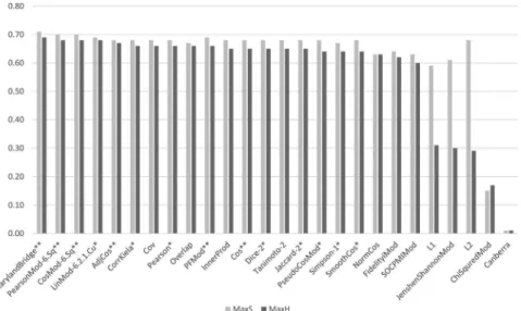
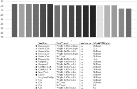
Most measures based on the inner product, also including correlation measures and statistical coeﬃcients, generally performed well (seeFigure 1). On the other hand, distance-based measures achieved relatively low H scores, mostly due to their low P scores. Measures designed for comparing probability distributions and for statistical hypothesis testing mostly also performed poorly. A large proportion of the best measures are modiﬁed variants of some existing measures, proposed by us (e.g. PearsonMod-6.Sq and CosMod-6.Sq).

The best measures achieved an H score close to 0.7, from which altogether 14 were selected to the second phase.

5.1.2. Weighting Schemes

The top of the table is clearly dominated by variants of PMI (see Figure 2). Beside these, some other complex information theoretic and statistical measures also scored high, while inter-rater reliability measures generally performed a little worse. Simple measures based on word-feature co-occurrence frequencies generally achieved relatively poor scores. Some of our newly proposed measures are among the best (e.g. WPMI-7 and PMIxLTU) .

The highest H scores are again close to 0.7. Altogether 15 measures were selected to the second phase.

Figure 1.First-phase performance of vector similarity measures using the DcBnc.

(12)

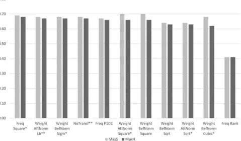
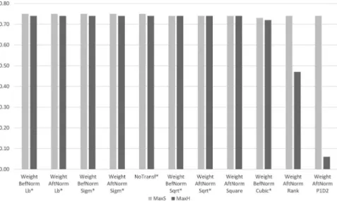
5.1.3. Feature Transformation

The results (see Figure 3) are rather mixed in case of this parameter.

Settings with all 4 major feature transformation categories have achieved good results, although with diﬀerent transformation functions in case of each. The best result was achieved using the newly proposed Square transformation function called on frequency counts before possible smoothing and normalization. Altogether 7 settings were selected to the second phase.

5.1.4. Dimensionality Reduction

Figure 4 shows that the best results were achieved by SVD with diﬀerent parameters, while no dimensionality reduction was superior to the other techniques. Altogether 3 settings were selected to the second phase.

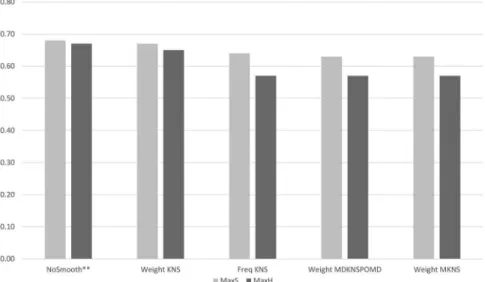
5.1.5. Smoothing

Smoothing seems to considerably worsen the results of DSMs (seeFigure 5), while posing signiﬁcant extra time and space complexity burden on them.

Therefore only the NoSmooth setting was selected for the next phase.

5.1.6. Vector Normalization

Many CPSs achieve the same results irrespective of which normalization technique is used, as a result of which the best scores of all 3 techniques are the same (see Figure 6). All of them were selected for the next phase.

Figure 2.First-phase performance of weighting schemes using the DcBnc.

(13)

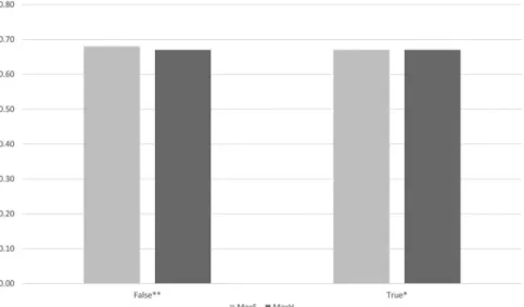
5.1.7. Filtering Stop-Words

As both options seem to achieve good results (see Figure 7), both were selected for the next phase.

Figure 3. First-phase performance of feature transformation techniques using the DcBnc.

Figure 4.First-phase performance of dimensionality reduction techniques using the DcBnc.

(14)

5.1.8. Minimum Limits on Word-Feature Tuple Frequencies

As employing minimum limits on word-feature tuple frequencies seems to deteriorate performance (see Figure 8), only the NoLimit option was selected for the second phase.

Figure 5.First-phase performance of smoothing techniques using the DcBnc.

Figure 6.First-phase performance of vector normalization techniques using the DcBnc.

(15)

5.1.9. Minimum Limits on Word-Feature Tuple Weights

Setting a minimum limit of 0.0 on word-feature tuple weights seems to be the best option (see Figure 9). Therefore this setting, together with the NoLimit option out of convention, was selected for the second phase.

Figure 7.First-phase performance achieved byﬁltering and notﬁltering stop-words using the DcBnc.

Figure 8. First-phase performance achieved by setting minimum limits on word- feature tuple frequencies using the DcBnc.

(16)

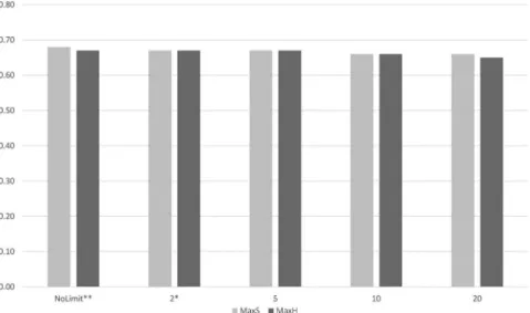
5.1.10. Minimum Limits on Feature Frequencies

As setting no or a very low limit on feature frequencies seems to achieve the best results (seeFigure 10), only 2 options were selected for the next phase.

5.2. Results Using the Semantic Vectors of Mikolov et al. (2013) 5.2.1. Vector Similarity Measures

These measures show very similar results using the Mv (seeFigure 11), as using the DcBnc. Measures based on the inner product, also including correlation measures and statistical coeﬃcients, achieved the highest H scores. Further, distance-based measures and measures designed for comparing probability distributions and for statistical hypothesis testing performed poorly most of the time. Again, some of our newly proposed measures were among the best.

The best measures achieved an H score around 0.75, from which altogether 18 were selected for the second phase.

5.2.2. Feature Transformation

The results (seeFigure 12) are rather mixed in case of this parameter using the Mv too, but resemble the results using the DcBnc more or less.

Altogether 8 settings were selected to the second phase.

Figure 9. First-phase performance achieved by setting minimum limits on word- feature tuple weights using the DcBnc.

(17)

5.2.3. Vector Normalization

Similarly as in case of the DcBnc, the best scores of both techniques (the NN option could not be tested with the Mv) are the same (seeFigure 13), and both of them were selected for the next phase.

Figure 10.First-phase performance achieved by the setting minimum limits on feature frequencies using the DcBnc.

Figure 11.First-phase performance of vector similarity measures using the Mv.

(18)

5.2.4. Minimum Limits on Word-Feature Tuple Weights

No limit or a minimum limit of −0.1 on word-feature tuple weights achieved the best results by far (see Figure 14). Therefore these, together with the 0.0 limit option out of convention, were selected for the second phase.

Figure 12.First-phase performance of feature transformation techniques using the Mv.

Figure 13.First-phase performance of vector normalization techniques using the Mv.

(19)

6. The Second Phase of the Heuristic Approach

The purpose of this phase was to determine what the best possible CPS is in case of CVBMs (using DcBnc) and PMs (using Mv) by testing all combinations of the selected settings for all parameters. A dataset (MD2) distinct from the one used in theﬁrst phase was used for evaluation.

In case of PMs, a full analysis was also feasible due to the lower number of parameters, therefore this was also done to validate the results.

Moreover, to even further verify the results, we have run a full heuristic analysis using the Sv too.

6.1. Results Using the Counts of Dobó & Csirik (2013) on the BNC With the settings of the 10 parameters selected in theﬁrst phase, altogether 71064 CPSs were tested. A small sample of these is presented inFigure 15.

The CPS with the best result will be referenced as BestCvbmDcBnc in the rest of the article. The WPMI-7 weighting scheme, proposed by us and part of BestCvbmDcBnc, is deﬁned as follows:

lb 1þfð;r;Þ fðw;r;w⁰Þ fðw;r;Þ fð;r;w⁰Þ

lb fð;r;Þ fðw;r;w⁰Þ fðw;r;Þ fð;r;w⁰Þ

(3) We also wanted to include the results achieved with the selected best CPS in case of PMs (seeFigure 16), run on the DcBnc. However, as only 4 out of 10 parameters could be used in case of PMs, the hypothetical best CPS of Figure 14. First-phase performance achieved by setting minimum limits on word- feature tuple weights using the Mv.

(20)

the 10 parameters were produced by changing the settings of these 4 parameters in BestCvbmDcBnc to the settings of the best method on PMs (included at the bottom ofFigure 15, and referenced as BestPmMvOnCvbm in the rest of the article).

Figure 15.Second-phase performance of CPSs using the DcBnc.

Figure 16.Performance of CPSs from the heuristic analysis in second phase using the Mv.

(21)

6.2. Results Using the Semantic Vectors of Mikolov et al. (2013) 6.2.1. Results Based on the Heuristic Tests

With the settings of the 4 parameters selected in the ﬁrst phase, altogether 864 CPSs were tested. A small sample of these is presented in Figure 16. The CPS with the best result will be referenced as BestPmMv in the rest of the article. SmoothCos, part of BestPmMv, is a similarity measure introduced by Riedl (2016).

The results achieved with the BestCvbmDcBnc, run on information extracted from Mv, are also included at the bottom of Figure 16 (please note that only 4 out of the 10 parameters could be used here). It will be referenced as BestCvbmDcBncOnPm in the rest of the article.

6.2.2. Veriﬁcation of the Heuristic Approach

By comparing the results of the full analysis using the Mv (seeFigure 17) with that of the heuristic analysis, we have discovered that the best 26 CPSs were the same using both analyses, which has highly exceeded our expectations.

As a result of the same two-phase heuristic analysis using the Sv as we have done using the Mv, we have got a rather diﬀerent best CPS (BestSv) than BestPmMv. However, they give very similar results, when using the same input and tested on the same dataset, as it will also be seen in Table 2.

Both these results give us a very strong veriﬁcation that the idea behind our heuristic approach was good, and that its results are reliable. Moreover, it also supports our assumption that a CPS working well on given input data also works well on other input data of the same type.

Figure 17.Performance of CPSs from the full analysis in second phase using the Mv.

(22)

7. Evaluation

7.1. Evaluation of Our Best Combinations of Parameter Settings on the MD2 Development Dataset

Our results on the MD2 dataset (see Figures 15 and 16) show that the BestCvbmDcBnc CPS, incorporating a novel weighting scheme, signiﬁ- cantly outperforms conventional variants (e.g. simple methods with cosine similarity and positive pointwise mutual information). Further, the novel CPS of BestPmMv also signiﬁcantly outperforms conventional ones.

Although the parameter settings of the BestCvbmDcBnc and BestPmMv CPSs highly resemble each other, their 4 mutual parameters do not have the exact same settings. Further, the two mixed CPSs (BestCvbmDcBncOnPm and BestPmMvOnCvbm) perform signiﬁcantly worse than the BestCvbmDcBnc and BestPmMv. Out of the BestCvbmDcBnc and BestPmMv variants the latter achieves considerably better results.

7.2. Evaluation of Our Best Combinations of Parameter Settings on the MT Dataset, Using Multiple Sources as Input

All 4 of our previously inspected CPSs have also been tested on the MT test dataset (seeTable 2). In some cases we have evaluated the same CPSs using multiple input data sources (i.e. diﬀerent extracted raw counts or diﬀerent semantic vectors).

As expected from the result on the MD2 dataset, the results of the Best PmMvUsingMvmodel are superior to that of the BestCvbmDcBncUsing- DcBnc model. As also anticipated, the mixed model using both the DcBnc

Table 2.Performance of our best models on the MT dataset. A model named XUsingY means the CPS X using Y as input data.

Parameter settings S H

CVBMs using solely distributional linguistic data

BestPmMvOnCvbmUsingDcBnc 0.39 0.37

BestCvbmDcBncUsingDcBnc 0.69 0.68

BestCvbmDcBncMinFFreq20UsingDcEw 0.74 0.72

BestCvbmDcBncUsingLcBnc 0.70 0.68

BestCvbmDcBncMinFFreq20UsingLcEw 0.75 0.73

BestCvbmDcBncUsingEcBnc 0.76 0.75

BestCvbmDcBncMinFFreq20UsingEcEw 0.78 0.76

PMs using solely distributional linguistic data

BestCvbmDcBncOnPmUsingMv 0.69 0.64

BestPmMvUsingMv 0.76 0.76

BestPmMvUsingPv 0.80 0.80

Other types of models

BestPmMvUsingSv 0.87 0.86

BestSvUsingSv 0.87 0.87

(23)

and the Mv as input (BestPmMvOnCvbmUsingDcBnc and BestCvbmDcBncOnPmUsingMv) achieved worse results than the non- mixed model using the same input data (BestCvbmDcBncUsingDcBnc and BestPmMvUsingMv, respectively) in all cases. On the other hand all count-vector-based and predictive CPSs performed well on all input data of the same type, as already supported for predictive CPSs by the results presented inSection 6.2.2.

When using the Ew as underlying corpus with the BestCvbmDcBnc CPS, we had to limit the features to those having a minimum frequency of 20 (MinFFreq20) due to computational reasons. Based on the result presented inSection 5.1.10 and also verified by additional tests, such a limitation has a negative impact on the results. Despite this negative effect, using the larger Ew corpus as input produced considerably better results, having the information extracted with either the Dc, Lc or Ec method. We were not able to do the same comparison in case of PMs, as all models used different input data, but most likely we would have come to the same conclusion as in case of CVBMs.

When using raw counts as input with the same underlying corpus in all cases, then the best results were achieved when using the Ec information extraction method, followed by the models using the Lc. In case of semantic vectors as input, the best results were achieved when using the Sv and Pv vectors, in that order.

As our best models achieved very similar results on all development and test datasets as well as using diﬀerent input data, we can conclude that there was no overﬁtting.

7.3. Comparison of Our Best Results with the State-Of-The-Art Beside the MT dataset, we have also run our best models on the MF dataset, and compared our results to that of state-of-the-art models inTable 3.

Our best PM achieves state-of-the-art results when using state-of-the-art semantic vectors as input. In case of CVBMs, our results are a little lower than current reported state-of-the-art. However, the underlying corpora used for our CVBMs are relatively small, while some others used hundreds of times larger corpora than ours. As the size of the used corpus has a large impact on the results, as also seen inTable 2, the results reported inTable 2 can only be viewed as supplementary results, while conclusions should not be taken from them.

Therefore, in order to be able to present a reliable comparison, we have done tests with multiple state-of-the-art models in such a way that the same input data was used for both those models and for our models too (seeTable 4). The input data tried included state-of-the-art semantic vectors as well as information extracted from diﬀerent corpora using state-of-the-art CVBMs.

(24)

In those cases where count-vector-based extracted information was used as input, all 10 of our inspected parameters could be tested. Where directly the obtained semantic vectors were used, only 4 parameters could be tested as the other parameters could have only been used during the construction of the vectors, which was already done. In case of the CVBM semantic vectors (Ev), this reduced the number of tested parameters from 10 to 4. In Table 3.Performance of our best models and some state-of-the-art systems on the test datasets. The results for the models marked with * come from reproductions of the given model by us, to be able to report all scores for those models too.

Test dataset MT MF

Evaluation measure S H S H

CVBMs using solely distributional linguistic data

Levy et al. (2015) – – 0.78 –

Pennington et al. (2014)* 0.80 0.80 0.80 0.80

Salle et al. (2018)* 0.81 0.81 0.81 0.81

BestCvbmDcBncMinFFreq20UsingEcEw 0.78 0.76 0.77 0.76

Baroni et al. (2014)* 0.80 0.79 0.80 0.79

Christopoulou et al. (2018) 0.84 – – –

BestPmMvUsingPv 0.80 0.80 0.80 0.80

Bruni et al. (2013) 0.78 – – –

De Deyne, Perfors, and Navarro (2017) – – 0.87 –

Speer et al. (2017)* 0.87 0.86 0.86 0.85

BestSvUsingSv 0.87 0.87 0.86 0.86

Table 4.Comparison of our best settings combinations with state-of-the-art models, with the original settings combination (OSC) proposed by the authors for those models, using the same input data for the OSCs and for our best CPSs, evaluated on the MT dataset.

Used input data Parameter settings # of tested parameters S H CVBMs using solely distributional linguistic data

LcBnc OSC – 0.64 0.63

BestCvbmDcBnc 10 0.70 0.68

LcEw OSC – 0.73 0.71

BestCvbmDcBncMinFFreq20 10 0.75 0.73

EcBnc OSC – 0.58 0.58

BestCvbmDcBnc 10 0.76 0.75

EcEw OSC – 0.62 0.62

BestCvbmDcBncMinFFreq20 10 0.78 0.76

Ev OSC – 0.81 0.81

BestPmMv 4 0.81 0.81

Bv OSC – 0.80 0.79

Pv OSC – 0.80 0.80

Sv OSC – 0.87 0.86

(25)

case of the other semantic vectors it did not result in any disadvantages, as in case of such models we could only use the same 4 parameters by default anyway.

In case of semantic vectors used as input, our results were always exactly the same as that of the original settings combination (OSC) proposed by the authors for the given model. On the other hand, when using the count- vector-based information extracted from diﬀerent corpora, we achieved considerably better results than the OSC proposed both by Levy et al. (2015) and by Salle et al. (2016) in their state-of-the-art model. During these tests too, using larger input corpora clearly improved the results.

8. Discussion

During our heuristic approach we were able toﬁnd such a novel combination of parameter settings using both the counts of Dobó & Csirik (2013) on the British National Corpus and the semantic vectors of Mikolov et al.

(2013), incorporating a novel weighting scheme in case of the former, that signiﬁcantly outperform conventional settings combinations.

Although these settings combinations resemble each other, it is clear from our results that different parameter settings have to be used in case of count- vector-based and predictive models. Most likely this is partially due to the fact that the settings of the different parameters influence each other, and in case of predictive models only 4 of the 10 parameters could be used. On the other hand, a settings combination working well using a given count-vector-based or predictive input also works well using other input of the same type.

It is easy to see that using a larger corpus as input for count-vector-based models produces considerably better results, despite having to reduce the number of features used due to computational reasons. This is most likely true for predictive models too.

Our best predictive model achieves considerably better results than our best count-vector-based model. This is most likely due to the approximately 1000 times larger corpus behind the former than behind the latter. We would expect that using a similarly large corpus with the count-vector- based model would greatly improve its results, but were not able to test this due to our limited resources.

Our most important tests were those where we used the same input data for state-of-the-art models and for our models too. Although we could signiﬁcantly improve on the results of conventional settings in case of the semantic vectors of Mikolov et al. (2013) as input, our results were always exactly the same as that of the state-of-the-art original settings combination proposed by the authors of the given model in case of all other semantic vectors. But as noted before, in these cases only 4 of our 10 examined parameters could be tested.

(26)

On the other hand, with our novel combination of the settings of the 10 parameters tested, we were able to considerably outperform the original settings combinations when extracted information of state-of-the-art count- vector-based models were used. These reﬂect our previous results and intuition, as experienced during our heuristic approach.

The best combinations of parameter settings found in the second phase of our heuristic approach are not simply the combinations of the best parameter settings found during theﬁrst phase, when the parameters were tested one by one. This clearly shows that our intuition was correct that the settings of the diﬀerent parameters are dependent on each other, and instead of testing the parameters separately they need to be tested together, also considering the interactions between them.

To sum up, the mainﬁndings of our analysis are summarized inTable 4, in which we have shown that we were able to ﬁnd such combinations of parameter settings that

•could considerably improve current state-of-the-art results when using raw counts as input and thus all 10 parameters could be optimized,

• perform exactly as well as current state-of-the-art models when using semantic vectors as input and thus only 4 out of 10 parameters could be optimized.

9. Conclusions

In this article, we have presented a very detailed and systematic analysis of the possible parameters used during the creation and comparison of feature vectors in DSMs, filling a serious research gap. We have identi- fied 10 important parameters of count-vector-based models and 4 relevant ones in case of predictive models, and tested numerous settings for all of them. Our analysis included novel parameters and novel parameter settings previously untested for DSMs, and tested all parameters simultaneously, thus also taking the possible interaction between the different parameters into account.

With our two-step heuristic approach we were searching for the best combinations of parameter settings, and were able tofind such novel ones, some of them also incorporating a novel weighting scheme, that signifi- cantly outperformed conventional combinations. Although we have used a heuristic approach for the search due to the vast number of possible combinations, we have been able to verify the validity of this approach and the reliability and soundness of its results. Further, we have also verified that a settings combination performing well on given input data also works well on other input data of the same type.

To be able to compare our results with the current state-of-the-art, we have run such tests where the same input data was used as input for both the current

(27)

state-of-the-art models and our models. In case of using raw counts as input and thus being able to optimize all 10 of our examined parameters, our best settings combinations contained a novel weighting scheme and achieved considerably better results than current state-of-the-art settings combinations. When using semantic vectors as input and thus only being able to optimize 4 out of 10 parameters, our best settings combinations achieved exactly the same results as the current state-of-the-art. Based on this we think that our analysis was success- ful, and we were able to present such a new weighting scheme and new combinations of parameter settings that can produce state-of-the-art results, and could be used in further models at least as well as current state-of-the-art settings combinations.

As it could be seen, the size of the input corpus, as well as the used information extraction method greatly inﬂuences the results, therefore we think that further research should be aimed in that direction.

We think that with this study we signiﬁcantly contributed to the better understanding of the working and properties of DSMs. Although fully reliable conclusions from our results can only be drawn with respect to DSMs, we think that similar conclusions would hold for other systems using vector space models too. So in our view our results could also be useful (with some reservations) outside the scope of DSMs, in case of other NLP and non-NLP problems using vector space models too.

Notes

1. https://code.google.com/archive/p/word2vec/.

2. https://bitbucket.org/omerlevy/hyperwords/.

3. https://github.com/alexandres/lexvec/.

4. https://github.com/stopwords-iso/.

Disclosure statement

No potential conﬂict of interest was reported by the authors.

ORCID

András Dobó http://orcid.org/0000-0002-8640-6073 János Csirik http://orcid.org/0000-0003-3870-0363

References

Aouicha, M. B., Hadj Taieb, M. A., & Hamadou, A. B. (2016). Taxonomy-based information content and wordnet-wiktionary-wikipedia glosses for semantic relatedness. Applied Intelligence, 45, 475–511.

(28)

Baroni, M., Dinu, G., & Kruszewski, G. (2014). Don’t count, predict! A systematic comparison of context-counting vs. context-predicting semantic vectors. In 52nd ACL (pp. 238–247). ACL. Stroudsburg PA.

Bruni, E., Tran, N. K., & Baroni, M. (2013). Multimodal distributional semantics.

Journal of Articiﬁal Intelligence Research, 48, 1–47.

Chen, S. F., & Goodman, J. (1999). An empirical study of smoothing techniques for language modeling. Computer Speech & Language, 13, 359–393.

Christopoulou, F., Briakou, E., Iosif, E., & Potamianos, A. (2018). Mixture of topic-based distributional semantic and aﬀective models. In 12th IEEE ICSC (pp. 203–210). IEEE.

Piscataway, NJ.

Church, K. W., & Hanks, P. (1990). Word association norms, mutual information, and lexicography. Computational Linguistics, 16, 22–29.

De Deyne, S., Perfors, A., & Navarro, D. J. (2017). Predicting human similarity judgments with distributional models: The value of word associations. In 26th IJCAI (pp. 4806–4810). IJCAI. Marina del Rey, CA.

Dobó, A. (2018). Multi-D kneser-ney smoothing preserving the original marginal distributions. Research in Computing Science, 147 (6), 11–25.

Dobó, A., & Csirik, J. (2013). Computing semantic similarity using large static corpora. In LNCS (Vol. 7741, pp. 491–502). Springer-Verlag. Berlin Heidelberg, Germany.

Evert, S. (2005). The Statistics of word cooccurrences word pairs and collocations (Ph.D. thesis). Universität Stuttgart. Stuttgart, Germany.

Islam, A., & Inkpen, D. (2008). Semantic text similarity using corpus-based word similarity and string similarity. ACM Transactions on Knowledge Discovery from Data, 2, 1–25.

Kiela, D., & Clark, S. (2014). A systematic study of semantic vector space model parameters. In 2nd CVSC at EACL (pp. 21–30). ACL. Stroudsburg PA.

Kneser, R., & Ney, H. (1995). Improved backing-oﬀfor n-gram language modeling.

In IEEE ICASSP (Vol. 1995, pp. 181–184). IEEE. Piscataway, NJ.

Lapesa, G., & Evert, S. (2014). A large scale evaluation of distributional semantic models: Parameters, interactions and model selection. Transactions of the Association for Computational Linguistics, 2, 531–545.

Levy, O., Goldberg, Y., & Dagan, I. (2015). Improving distributional similarity with lessons learned from word embeddings. Transactions of the Association for Computational Linguistics, 3, 211–225.

Melamud, O., Levy, O., & Dagan, I. (2015). A simple word embedding model for lexical substitution. In 1st CVSC at NAACL (pp. 1–7). ACL. Stroudsburg PA.

Mikolov, T., Corrado, G., Chen, K., & Dean, J. (2013). Eﬃcient estimation of word representations in vector space. In ICLR (Vol. 2013, pp. 1–12). ICLR. Scottsdale, AZ.

Pennington, J., Socher, R., & Manning, C. D. (2014). GloVe: Global vectors for word representation. In EMNLP (Vol. 2014, pp. 1532–1543). ACL. Stroudsburg PA.

Riedl, M. (2016). Unsupervised Methods for Learning and Using Semantics of Natural Language. Ph.D. thesis Technischen Universität Darmstadt.

Salle, A., Idiart, M., & Villavicencio, A. (2016). Matrix factorization using window sampling and negative sampling for improved word representations. In 54th ACL (pp. 419). ACL. Stroudsburg PA.

Salle, A., Idiart, M., & Villavicencio, A. (2018). LexVec. Retrieved July 04, 2018, fromhttps://github.com/alexandres/lexvec/blob/master/README.md

(29)

Santus, E., Chersoni, E., Lenci, A., Huang, C.-R., & Blache, P. (2016). Testing APSyn against vector cosine on similarity estimation. In 30th PACLIC (pp. 229–238). Kyung Hee University. Seoul, South Korea.

Speer, R., Chin, J., & Havasi, C. (2017). ConceptNet 5.5: An open multilingual graph of general knowledge. In 31st AAAI (pp. 4444–4451). AAAI Press. Palo Alto, CA.

Vakulenko, M. (2018). Calculation of semantic distances between words: From synonymy to antonymy. Journal of Quantitative Linguistics, 1–13.

Weeds, J. E. (2003). Measures and applications of lexical distributional similarity (Ph.D. thesis). University of Sussex. Falmer, United Kingdom.