METHODS OF MODELLING THE FUTURE SHIFT OF THE SO CALLED MOESZ-LINE
BEDE-FAZEKAS,Á.
Corvinus University of Budapest, Department of Garden and Open Space Design 1118 Budapest, Villányi út 29-43., Hungary
(phone: +36-20-367-5366) e-mail: bfakos@gmail.com
(Received 3rd March 2012; accepted 8th May 2012)
Abstract. It is important to the landscape architects to become acquainted with the results of the regional climate models so they can adapt to the warmer and more arid future climate. Modelling the potential distribution area of certain plants, which was the theme of our former research, can be a convenient method to visualize the effects of the climate change. A similar but slightly better method is modelling the Moesz-line, which gives information on distribution and usability of numerous plants simultaneously.
Our aim is to display the results on maps and compare the different modelling methods (Line modelling, Distribution modelling, Isotherm modelling). The results are spectacular and meet our expectations:
according to two of the three tested methods the Moesz-line will shift from South Slovakia to Central Poland in the next 60 years.
Keywords: Gusztáv Moesz, climate change, GIS, distributional range, climate shift
Introduction
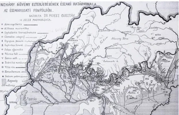
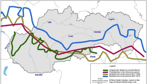
Gusztáv Moesz (1873-1946) was a botanist, mycologist and museologist who obtained an international reputation by his mycology researches. The most important observation for the Central-European botany and landscape architecture he made was published more than 100 years ago. He discovered that certain plants share a common northern distribution border and this coincides with the line of vine cultivation (Moesz, 1911). This line lying in the Northern Carpathians is named after him. The old maps (Fig. 1 and Fig. 2) primarily have a historical importance. Subordinately, the map showed in Fig. 1 is the most accurate source of the distributions used in this research.
Fig. 2 shows the Moesz-line updated by the author.
The predicted shift of the Moesz-line in the 21st century and the research methods are summarized in this paper. Our preliminary expectation was that the Moesz-line will shift towards Poland in two nearly equal steps in the modelled future periods of 2011- 2040 and 2041-2070.
Figure 1. ‘Northern border of the distribution of some plant species in the Northwest Highlands’. The map of the distribution of 12 taxa and the vine cultivation area with the former
frontier of the country and hydrography (Moesz, 1911; with some retouching).
Figure 2. ‘Border line between the Tatra-Fatra and the Pannonian floristic region’ in a hydrographic chart. The line drawn by Moesz is the red one (Moesz, 1911; retouched and
updated by the author).
Review of literature
The importance of the Moesz-line on botany and landscape architecture
The Moesz-line is hardly ever used in international scientific publications due to its local importance. However, extending the northern line of vine cultivation towards East and West, one can obtain the extension of the Moesz-line, which will be corresponding to the northern distribution border of some other species such as Grape Hyacinth (Muscari botryoides (L.) Mill.; Somlyay, 2003), too. The Moesz-line modelling is important for the entire Continent because it is illustrative for the indigenous and ornamental plants not only of the Carpathian Basin.
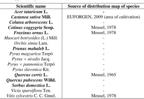
Originally Moesz included 12 wild plants and the cultivated grapevine (Vitis vinifera L.) in his research. Table 1 shows the originally used and the accepted scientific names of the observed plans and the sources of the distributional maps (Moesz, 1911;
Meusel et al., 1965; Meusel et al., 1978; Meusel and Jäger, 1992; Tutin et al., 1964;
EUFORGEN, 2009). Species used as ornamental plants in Hungary are highlighted (Bede-Fazekas and Gerzson, 2011).
Table 1. The list of the 12+1 species originally used for drawing the Moesz-line with the sources of the distribution maps used in our research. The species used as ornamental plants in Hungary are highlighted. Accepted scientific names are according to GRIN (2012), supported by IPNI (2005) and Priszter (1998).
Scientific name used by Gusztáv Moesz
Accepted scientific name Source of distribution map of species
Aira capillaria Aira elegantissima Schur Moesz, 1911 (Meusel, 1965) Althaea micrantha Althaea officinalis L. Moesz, 1911 (Meusel, 1978)
Cephalaria transsilvanica
Cephalaria transsylvanica (L.) Roem. & Schult.
Moesz, 1911
Clematis integrifolia Clematis integrifolia L. Moesz, 1911 (Tutin et al., 1964)
Eryngium planum Eryngium planum L. Moesz, 1911
Euphorbia gerardiana Euphorbia seguieriana Neck. Moesz, 1911 (Meusel, 1978) Galega officinalis Galega officinalis L. Moesz, 1911 Galium pedemontanum Cruciata pedemontana
(Bellardi) Ehrend.
Moesz, 1911 Phlomis tuberosa Phlomis tuberosa L. Moesz, 1911 (Meusel, 1978)
Salvia aethiopis Salvia aethiopis L. Moesz, 1911 Sideritis montana Sideritis montana L. Moesz, 1911 Xeranthemum annuum Xeranthemum annuum L. Meusel, 1992 (Moesz, 1911)
Vitis vinifera Vitis vinifera L. Moesz, 1911 (area of cultivation)
The importance of Moesz-line is, for the landscape architecture, beyond the investigation of the original 12 species. It plays an important role in agriculture by determining the cultivation area of vine. Moreover, Moesz-line also demonstrates the northern border of the spread of some important species that have been added later to this concept. Among these are the Bladder Senna (Colutea arborescens L.; Csiky, 2003), Chestnut (Castanea sativa Mill.; Bartha, 2007), Pubescent Oak (Quercus pubescens Willd.; Csapody, 1932; Kárpáti, 1958; Kézdy, 2001; Bartha, 2002), Service Tree (Sorbus domestica L.; Végvári, 2000), and some pear species (Terpó, 1992).
Table 2 lists the species that have their distribution border near to the Moesz-line.
Species having a key role in landscape planning are highlighted. Table 2 contains the source of the distribution maps, too.
Table 2. List of the taxa with distribution bound to the Moesz-line. Species having importance in landscape architecture are highlighted. Scientific names are according to GRIN (2012), supported by IPNI (2005).
Scientific name Source of distribution map of species
Acer tataricum L. -
Castanea sativa Mill. EUFORGEN, 2009 (area of cultivation)
Colutea arborescens L. -
Cotinus coggygria Scop. Meusel, 1978
Fraxinus ornus L. Meusel, 1978
Muscari botryoides (L.) Mill. -
Orchis simia Lam. -
Prunus mahaleb L. -
Pyrus magyarica Terpó -
Pyrus × nivalis Jacq. -
Pyrus × pannonica Terpó -
Pyrus slavonica Kit. -
Quercus cerris L. Meusel, 1965
Quercus pubescens Willd. -
Sorbus domestica L. -
Vicia sparsiflora Ten. -
Vitis sylvestris C. C. Gmel. Meusel, 1978
Visualization of the climate change and ecological modelling
According to the regional climate models the Carpathian Basin will become warmer and drier in the next century, and the extreme precipitations will occur more frequently during the hotter period of the year (Bartholy and Pongrácz, 2008). This will bring a challenging situation for the landscape designers who will have to face and have to be prepared to deal with this issue well in advance. The landscape designers can slightly change the climate (primarily the microclimate), chiefly they can adapt to it so proper adaptation has to be emphasized. To implement the best adaptation policy it is essential to get to know the expected climate of a future period. It is important in case of the landscape designing, horticulture and dendrology, to know the expected natural vegetation and adaptable ornamental plants.
In case of trees the development and growing period can be up to 30 years, so it is high time to address this issue with some easy-to-understand but effective visualization for expected future climate (Sheppard, 2005). In our research the shift of the climate is modelled with the visualization of the predicted Moesz-line. It can serve as an alternative for the modelling of geographically analogous regions (Horváth, 2008). It is necessary to stress that the shift of the Moesz-line primarily affects the Slovakian and Polish landscape architecture by direct means. However, the experiences of the Hungarian landscape architecture, dendrology and ornamental plant usage can help these countries to adapt to the changing climate. Thus, it is the task of our profession to collect and hand over the accumulated knowledge base.
We are unaware of any former ecological modelling research that can be bound to the Moesz-line. However, there are some publications that have similarities to the current research: either in the methodology or in the results. In the Central European region the impacts of the climate change on the distribution of the Sessile Oak was discussed by Czúcz et al. (2011). The distribution of the European Beech was researched by Führer and Mátyás (2006). Czúcz (2010) gives a full synopsis of the impacts of climate change on the Hungarian natural habitats. Bede-Fazekas (2011)
modelled the distribution of some Mediterranean species that can have ornamental importance in Hungary in the future. There are some other researches beyond the Central European region. Leng et al. (2008) modelled the distribution of Dahurian Larch, Korean Larch and Prince Rupprecht Larch according to three different climate scenarios. Iverson and Prasad (1998) predicted the abundance of 80 species of the United States. Sabaté et al. (2002) modelled the distribution of five different species in the Mediterranean region according to the HadCM2 model. Iverson et al. (1999) researched the predicted distribution of Virginia Pine under two scenarios of climate change. Bakkenes et al. (2006) made a comparison of the modelling results of different climate scenarios. Rotenberry et al. (2006) illustrates his ecological niche modelling approach with the distribution of California Gnatcatcher. Our research has some essential resemblance to Rotenberry’s research, for example in the use of the limiting factors. Guisan and Zimmermann (2000) give a good summary of different ecological modelling methods. Thuiller et al. (2008) points some imperfections of the widely used ecological models. There are some modelling softwares and mellow methods (Carpenter et al., 1993; Pearson et al., 2002; Li et al., 2008) developed for such modelling purposes. The enumeration is, however, not complete, ecological modelling has much wider range of literature.
Materials and methods Methods of modelling
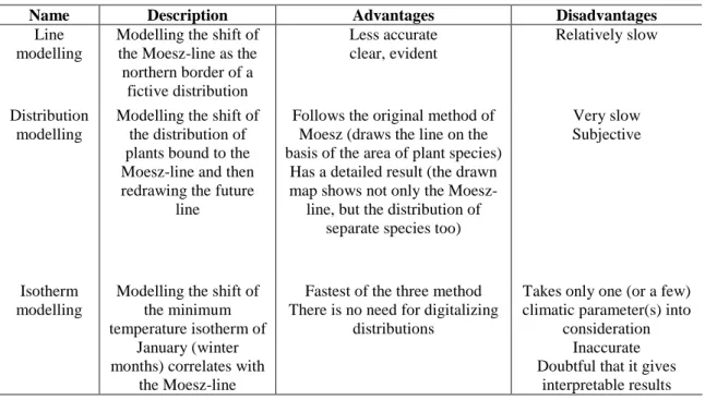
The expected shift of the Moesz-line can be modelled in numerous ways. In our research three methods were applied. Table 3 summarizes the characteristics of the methods and shows their advantages and disadvantages.
Table 3. Methods of the Moesz-line modelling used in our research with their advantages and disadvantages. The quickness of a certain method has an importance if the research is repeated (with other meteorological input or with refined sub-methods) or tested on other subject.
Name Description Advantages Disadvantages
Line modelling
Modelling the shift of the Moesz-line as the northern border of a
fictive distribution
Less accurate clear, evident
Relatively slow
Distribution modelling
Modelling the shift of the distribution of plants bound to the Moesz-line and then redrawing the future
line
Follows the original method of Moesz (draws the line on the basis of the area of plant species)
Has a detailed result (the drawn map shows not only the Moesz-
line, but the distribution of separate species too)
Very slow Subjective
Isotherm modelling
Modelling the shift of the minimum temperature isotherm of
January (winter months) correlates with
the Moesz-line
Fastest of the three method There is no need for digitalizing
distributions
Takes only one (or a few) climatic parameter(s) into
consideration Inaccurate Doubtful that it gives
interpretable results
All three methods were applied on the REMO ENSEMBLES RT3 climate model (ENSEMBLES, 2012) which contains data of a 25-km horizontal grid cell resolution of Europe (170×190 points). The reference period was 1961-1990 and the forecasted periods were between 2011-2040 and 2041-2070 according to the A1B IPCC SRES scenario. The A1 storyline and scenario family describes a future world of very rapid economic growth, global population that peaks in mid-century and declines thereafter, and the rapid introduction of new and more efficient technologies. Major underlying themes are convergence among regions, capacity building, and increased cultural and social interactions, with a substantial reduction in regional differences in per capita income. A1B scenario is one of the three from A1 scenario family. It describes a balance across all sources of energy system. (Nakicenovic and Swart., 2000).
The modelling was performed by the ESRI ArcGIS (Geographic Information System) software. For all three methods interpolation was necessary to create continuous data from the discrete dataset of the climate model. For this the Inverse Distance Weighted procedure of the Spatial Analyst extension was used. The given output cell size was 0.11 with a power of 2 and 12 searching points. No DTM (Digital Terrain Model) was used for the accurate interpolation. The horizontal resolution of the original climate model determined the precision of the future dataset; thus, using DTM could not really make the model more accurate.
The Isotherm modelling is the most simple of the three methods and it is not a real modelling method. Its essence is to find the minimum temperature isotherm that correlates the Moesz-line and follow the shift of this isotherm based on the meteorological dataset. It takes only one – or a few – climate parameter into consideration, thus, it is the most unreliable method. Line modelling is a more detailed method. It creates a fictive distribution (for a non-existent ‘Moesz plant’) that has a northern border equivalent to the Moesz-line. The model is executed on this distribution. The most complex but the slowest of the three methods is Distribution modelling. It runs the climate model on the distributions of 18 species and draws the predicted Moesz-line on the basis of the modelled distributions. This method follows the original way of drawing the Moesz-line in a way that it also bases on plant distributions. In our research geographical averaging methods were not used, so Distribution modelling is inaccurate from this point of view. (The whole modelling procedure contains so much subjectivity that there is no sense in applying geographical averaging methods on the last step.)
Line modelling and Distribution modelling
As a preparation for the Line modelling and the Distribution modelling, the original maps of Moesz were digitized and georeferenced using 20-25 control points (frontiers and rivers). For the Distribution modelling it was necessary to digitize the areas of each plant, since only the EUFORGEN data contained spatial coordinates. We did not consider the entire distribution of plants. Only the northern segment of the area was taken into consideration. (Additional limitation to the segment was that it did not spread to the south more than the fictive distribution bound to the ‘Moesz-plant’, and was located in the Carpathian Basin). Since only the northern borders were modelled, this did not modify the result at all.
Three parameters of the climate model were used: monthly average temperature, monthly minimum temperature and monthly total precipitation. All the temperature data of the 12 months were used. From the precipitation data only the total rainfall in the
vegetation period (April-September) was considered because it had been observed in former similar distribution models that if all of the precipitation data was taken into consideration the results could not be evaluated. Due to the climate change, the precipitation zones would shift to the north with different rates than the temperatures (Bede-Fazekas, 2011). However, the model can be further refined by using additional precipitation data. A more detailed model can be created with operating other climatic parameters such as heat sum.
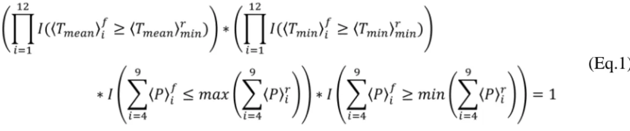
The minimum of the monthly average temperatures (1×12 parameters) and the minimum of the monthly minimum temperatures (1×12 parameters) were used (since the northern border was modelled) together with the upper and lower values of the total rainfall in the vegetation period (2×1 parameters). So, altogether 26 different logical conditions had to be fulfilled for a given spatial point to satisfy the climatic conditions.
The next equation summarizes these mathematical conditions.
(Eq.1)
In Equation 1 the indicator function I(λ) takes the value of 1 if the condition for λ is true, otherwise it takes the value of 0. The symbol r means the reference period, f stands for future period, i is the running variable (through the months).
Figure 3. An example of the distribution modelling (Sideritis montana L.). The map shows Central Europe with frontiers. The key for colours: green – actual distribution, red – modelled
distribution in the reference period, yellow – modelled distribution in the period 2011-2040, pink – modelled distribution in the period 2041-2070
From the individual areas of distributions (and in the Line modelling from the fictive distribution bound to the Moesz-line) we have selected 26 extreme values (25 minimums, 1 maximum) that belong to the 25 parameters and we run the modelling for the two future periods (Fig. 3) based on these extremities. Actually, this model displays the areas of those climatic conditions the given plant can tolerate but not it’s real distribution area. Since just parts of the real areas were chosen only the northern border of the modelled areas will give interpretable result. We have not dealt with edafic and microclimatic data in this research. By modelling the reference period we aimed to display the difference between the real distribution area and the potential distribution area predicted by the model. Thus, the models run for the reference period can validate (and make able to evaluate) the methods.
In the second type of modelling (Distribution modelling) we have analyzed the possible distribution of the species originally used for drawing the Moesz-line (Table 1) and the 5 species bound afterwards (Castanea sativa, Cotinus coggygria, Fraxinus ornus, Quercus cerris and Vitis sylvestris).
For one certain species (or the ‘Moesz-plant’) the detailed method of modelling was the following. Before the interpolation explained previously, the rainfall data of the vegetation period was summarized to a new field (column) with the Field Calculator procedure of the attribute table displayer of the GIS software. After the interpolation (so the base data of the research were the interpolated ones) we used the Zonal Statistics procedure of the Spatial Analyst extension on all the 25 parameters. The output table was set as temporary, since the minimum temperature and the minimum and maximum rainfall data were copied to a Microsoft Excel spreadsheet. From the copied data with the string concatenation and other string functions of Excel the appropriate formulas were created for the next step (for the reference period and the two future periods). Then we started the Raster Calculator procedure of the Spatial Analyst extension of ArcGIS, using the three formulas concatenated with Excel. From the drawn temporary raster files we selected the entities with the value ‘true’ (or 1) and created shapefiles of the modelled distributions. The Raster to Features conversation tool of the Spatial Analyst extension was used for this. The northern borders of the shapes were finally redrawn on base map, using Adobe Photoshop software. The legend was created with Photoshop too.
Isotherm modelling
The third method, the Isotherm modelling has three simple steps. First, we drew some isotherms of the reference period by the Surface Analysis/Contour procedure of the Spatial Analyst extension of ArcGIS. We choose the one most coincident with the original Moesz-line. In the second step we drew the isotherm of the same temperature based on the future datasets. Finally, we plot the isotherms on one map.
Isotherm modelling has a great similarity with the hardiness zones. USDA-zones, or hardiness zones, have a high importance in dendrology. It was developed by the Department of Agriculture of the United States (USDA). It classifies the ornamental plant species by their winter hardiness. The species are ranked among the 26 zones called 0a, 0b, 1a to 12b. The zones are based on the absolute minimum temperature; the lower number the zone have, the more hardy the plant is.
However, in our research we have only used the average minimum temperatures of January instead of the minimum temperature of the winter because in the Central
European region January is the coldest month. Also by this reduction we could benefit the main advantage of this method: simplicity.
Nevertheless, the most significant difference is that, instead of the absolute minimums used for the USDA-zones, the average minimums were accessible from this climate model for us. Likely for the Submediterranean flora the absolute minimum temperature has a higher importance but neither has it described the proper climatic requirements of the plants.
Results
Line modelling
According to the results of Line modelling (Fig. 4 and Fig. 5) the modelled Moesz- line for the reference period follows the original Moesz-curve so it shows a really good coherent result regarding the spatial resolution of the model. However, the predicted change of the Moesz-line for the period of 2011-2040 – unexpectedly – does not show a great shift to the north. Moreover, the east part of the Moesz-line between the cities of Rimavská Sobota and Tisovec (Slovakia), in the period of 2011-2040 is expected to lie slightly to the south of the line of the reference period. From the east to Rožňava (Slovakia) the modelled line cannot shift to the north of the original line. This result needs further investigation; however, it is suspected that the lower bound of the rainfall of the vegetation period pushes this line in the section under discussion to the south more than was expected.
Figure 4. The results of the line modelling zoomed into Slovakia, printed on a hydrographic chart with country frontiers
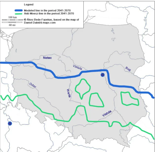
Even so, in the run for the period of 2041-2070, the results clearly show the expected shift of the Moesz-line towards the north. Two, or in other interpretation three different sections can be distinguished. First of all, in the Carpathian Mountains it moves to higher regions (to the north, Fig. 4) and from the north of the Carpathian Mountains it reaches Poland (Fig. 5). Naturally, an anti-Moesz-line is formed that bounds the
climatically optimal regions of Poland to the south (towards the Carpathians). The results coincide with the modelling of geographically analogue regions (Horváth, 2008).
The southern part of the new Moesz-line connects Brno and Zlín (Czech Republic), Trenčín, Zvolen, Lučenec, Kosice, Homenne (Slovakia), Soiva (Ukraine) and Bacău (Romania). The northern line connects Berlin (Germany), Poznań, Warsaw, Garwolin, Włodawa (Poland), Novohrad-Volinszkij and Bila Cerkva (Ukraine). The anti-Moesz- line joins Dresden (Germany), Bolesławiec, Rybnik, Częstochowa, Kraków (Poland) and Lviv (Ukraine).
Figure 5. The results of the line modelling zoomed into Poland, printed on a hydrographic chart with country frontiers. Territories between the blue and green lines are predicted to be the
ones equivalent to the territories currently situated to the south of the Moesz-line
Distribution modelling
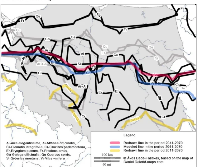
Figure 6. The modelled distribution of the species (gray: 2011-2040, black: 2041-2070), and the redrawn Moesz-lines, printed on a hydrographic chart with country frontiers
Distribution modelling – as it was expected – gives a more detailed result of the predicted shift of the Moesz-line (Fig. 6). Some species got separated from the others, the distribution of some species shifted to the north of the Carpathians as „early” as 2011-2040 and some of the plants have remained only on the southern parts of the Carpathians even in the period 2041-2070 (Table 4). It can be stated that the 12+1 original plants that determined the Moesz-line have produced a more coherent shift of distributions than those plants which were later added to the concept of Moesz-line. The distribution of the Manna Ash (Fraxinus ornus L.) and the Turkey Oak (Quercus cerris L.) is expected to shift to the north the most and only these two species will show a direct connection between the Slovakian and Polish modelled areas through the Carpathians. In addition to this, it can be stated that the Common Grape Vine (Vitis vinifera L.) and the Mountain Tea (Sideritis montana L.) will mostly follow the northern line obtained by the Line modelling method between 2041-2070.
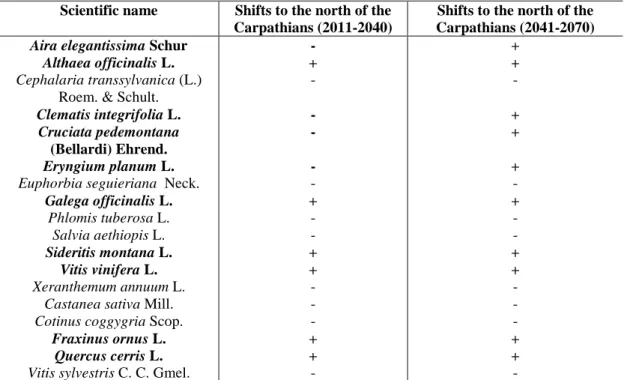
Table 4. The modelled species and their presence on the northern side of the Carpathians.
The bold typed ones shift to Poland at latest in the period of 2041-2070 Scientific name Shifts to the north of the
Carpathians (2011-2040)
Shifts to the north of the Carpathians (2041-2070)
Aira elegantissima Schur - +
Althaea officinalis L. + +
Cephalaria transsylvanica (L.) Roem. & Schult.
- -
Clematis integrifolia L. - +
Cruciata pedemontana (Bellardi) Ehrend.
- +
Eryngium planum L. - +
Euphorbia seguieriana Neck. - -
Galega officinalis L. + +
Phlomis tuberosa L. - -
Salvia aethiopis L. - -
Sideritis montana L. + +
Vitis vinifera L. + +
Xeranthemum annuum L. - -
Castanea sativa Mill. - -
Cotinus coggygria Scop. - -
Fraxinus ornus L. + +
Quercus cerris L. + +
Vitis sylvestris C. C. Gmel. - -
Comparing this to the results of the Line modelling, we can observe that in the period of 2011-2040 the Moesz-line is expected to pass over the Carpathians although the observed plants will only form some isolated or disconnected distribution regions. On the other hand, the Line modelling method has not predicted the future occurrence of the Moesz-line over the Carpathians. Distribution modelling and Line modelling have given almost the same results for the far future period, although the former displays the future Moesz-line slightly more to the north. The Slovakian segments of modelled line are not displayed separately, since it has produced, considering the horizontal resolution of the climate model, almost identical results with the Line modelling method.
Isotherm modelling
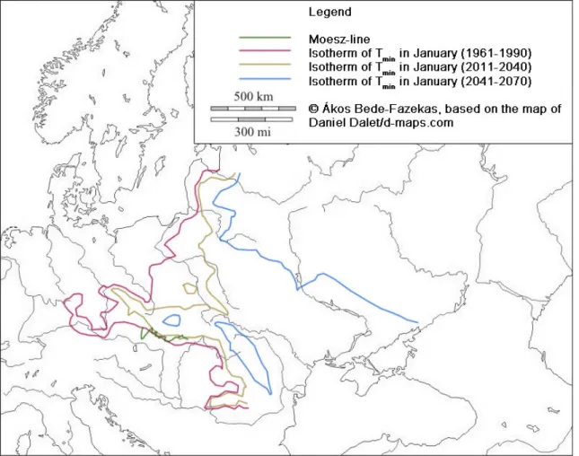
The Isotherm modelling has produced weaker results than it had been expected (Fig. 7). The isotherm of the average minimum temperature in January (-3.86°C) which mostly coincides with the Moesz-line in the reference period, oversteps the Carpathians in the reference period already. Moreover, the position of the curve is not parallel with the Carpathians but perpendicular. Probably, it is due to the climate balancing effect of the sea nearby. However, it cannot be taken into consideration since the Moesz-line is much more exposed to the continental climate impacts. So we can conclude that Isotherm modelling is not too useful for predicting the future shift of certain plants or the Moesz-line – no matter if we use the winter minimum or a monthly minimum temperature. One can observe that in the period of 2011-2040 the Carpathians will make a separating blockage but in the period of 2041-2070 – in terms of the isotherm of January – it will ensure free passage for the species. Due to the above mentioned problems we did not continue to evaluate the results of the Isotherm modelling further more.
Figure 7. The shift of the minimum temperature isotherm of January
Discussion
In this research three different methods were tested to predict the future shift of the Moesz-line due to climate change. The evaluation of them can be seen in Table 5.
Table 5. The evaluation of the methods used in our research
Name Usable Gives results according to
expectations
Line modelling + - (2011-2040)
+ (2041-2070)
Distribution modelling + +
Isotherm modelling - - (It was expected to get doubtful results but not get unusable results.)
It can be stated that the shift of the line toward north is smaller for the period of 2011-2040 than we expected, while for 2041-2070 it coincides with the pre-estimation.
We think the results of this research are worth presenting to the landscape architects and botanists. We can observe the expected change of climate in the next 60 years according to the A1B climate scenario.
In summary we can say that the Line modelling and Distribution modelling produced very similar results for 2041-2071. However, for the period of 2011-2040 only
Distribution modelling predicted possible shift to the north of the Carpathians. In spite of this the Distribution modelling does not give significantly more information than Line modelling. Nevertheless, the procedure takes a lot of time and it is fairly difficult to model so many different species separately. The only reason to use Distribution modelling is the tradition and scientific respect towards Moesz’s work, otherwise there is very little practical reason. The Isotherm modelling produced doubtful predictions and it worked even weaker than expected. As an overall conclusion we found the first method to be the most effective and reliable.
The shortcomings of the methods are that they select only a few of the infinite combinations of the finite climate parameters and the selection is arbitrary. The further improvement of such modelling could be based on more advanced statistical methods (which make the selection easier and more objective), or could use artificial intelligence methods. Among them (decision tree, evolutionary algorithm, and artificial neural network) the application of neural networks seems to be the best solution. There are some researches (Carpenter et al., 1999; Özesmi and Özesmi, 1999; Hilbert and Muyzenberg, 1999; Özesmi et al., 2006) on the subject of floristic modelling with artificial neural networks that have some similarities with this approach.
Acknowledgements. Special thanks to Mária Höhn (Corvinus University of Budapest, Department of Botany), Gábor Bőhm, Levente Horváth (Corvinus University of Budapest, Department of Mathematics and Informatics) and Anna Czinkóczky (Corvinus University of Budapest, Landscape and Settlement Analytic Laboratory) for their assistance. Heartfelt thanks to the referees for their substantial explanatory comments. The research was supported by Project TÁMOP-4.2.1/B-09/1/KMR-2010-0005. The ENSEMBLES data used in this work was funded by the EU FP6 Integrated Project ENSEMBLES (Contract number 505539) whose support is gratefully acknowledged.
REFERENCES
[1] Bakkenes, M., Eickhout, B., Alkemade, R. (2006): Impacts of different climate stabilisation scenarios on plant species in Europe. – Global Environmental Change 16(1):
19-28.
[2] Bartha, D. (2002): A molyhos tölgyek (Quercus pubescens agg.) botanikai jellemzése. – Erdészeti Lapok 137(1): 7-8.
[3] Bartha, D. (2007): A szelídgesztenye (Castanea sativa) botanikai jellemzése. – Erdészeti Lapok 142(1): 14-16.
[4] Bartholy, J., Pongrácz, R. (2008): Regionális éghajlatváltozás elemzése a Kárpát- medence térségére. – In: Harnos, Zs., Csete, L. (eds) Klímaváltozás: környezet – kockázat – társadalom. Szaktudás Kiadó Ház, Budapest
[5] Bede-Fazekas, Á., Gerzson, L. (2011): Évelő dísznövények kompendiuma kladisztikai rendszertan szerint. – Assa-Divi, Budapest
[6] Bede-Fazekas, Á. (2011): Impression of the global climate change on the ornamental plant usage in Hungary. – Acta Universitatis Sapientiae Agriculture and Environment 3(1): 211-220.
[7] Carpenter, G., Gillison, A. N., Winter, J. (1993): DOMAIN: a flexible modelling procedure for mapping potential distributions of plants and animals. – Biodiversity and Conservation 2(1): 667-680.
[8] Carpenter, G.A., Gopal, S., Macomber, S., Martens, S., Woodcock, C.E., Franklin, J.
(1999): A Neural Network Method for Efficient Vegetation Mapping. – Remote Sensing of Environment 70(3): 326-338.
[9] Csapody V. (1932): Mediterrán elemek a magyar flórában. – Dissertation. Szegedi Tudományegyetem, Szeged
[10] Csiky J. (2003): A Nógrád-Gömöri bazaltvidék flórája és vegetációja. – Tilia 11(1): 167- 301.
[11] Czúcz B. (2010): Az éghajlatváltozás hazai természetközeli élőhelyekre gyakorolt hatásainak modellezése. – Dissertation, Budapesti Corvinus Egyetem, Budapest
[12] Czúcz, B., Gálhidy, L. Mátyás, Cs. (2011): Present and forecasted xeric climatic limits of beech and sessile oak distribution at low altitudes in Central Europe. – Annals of Forest Science 68(1): 99-108.
[13] ENSEMBLES (2012): The ENSEMBLES project RT3. – http://ensemblesrt3.dmi.dk;
2012.04.04.
[14] EUFORGEN (2009): Distribution map of Chestnut (Castanea sativa). – http://www.euforgen.org
[15] Führer, E., Mátyás, Cs. (2006): A klímaváltozás hatása a hazai erdőtakaróra. – AGRO 21 Füzetek, 48(1):34-38.
[16] GRIN (2012): Germplasm Resources Information Network of the United States Department of Agriculture's (USDA's) Agricultural Research Service (ARS). – http://www.ars-grin.gov/cgi-bin/npgs/html/taxgenform.pl?language=en; 2012.04.04.
[17] Guisan, A., Zimmermann, N.E. (2000): Predictive habitat distribution models in ecology.
– Ecological Modelling 135(2-3): 147-186.
[18] Hilbert, D.W., Muyzenberg, J.V.D. (1999): Using an artificial neural network to characterize the relative suitability of environments for forest types in a complex tropical vegetation mosaic. – Diversity and Distributions 5(6): 263-274.
[19] Horváth L., (2008): A földrajzi analógia alkalmazása klímaszcenáriók vizsgálatában. – In:
Harnos Zs., Csete L. (eds) Klímaváltozás: környezet – kockázat – társadalom. Szaktudás Kiadó Ház, Budapest
[20] IPNI (2005): International Plant Names Index. – http://ww.ipni.org/ipni; 2012.04.04.
[21] Iverson, L.R., Prasad, A.M. (1998): Predicting Abundance of 80 Tree Species Following Climate Change in the Eastern United States. – Ecological Monographs 68(4): 465-485.
[22] Iverson, L.R., Prasad, A., Schwartz, M.W. (1999): Modelling potential future individual tree-species distributions in the eastern United States under a climate change scenario: a case study with Pinus virginiana. – Ecological Modelling 115(1): 77-93.
[23] Kárpáti Z. (1958): A természetes növénytakaró és a kertészeti termesztés közti összefüggés Sopron környékén. – Soproni Szemle 12(3): 30-54.
[24] Kézdy P. (2001): Taxonómiai vizsgálatok a hazai molyhos tölgy alakkörön (Quercus pubescens s. l.). – Dissertation. Nyugat-Magyarországi Egyetem, Soproni Egyetemi Karok, Sopron
[25] Leng, W., He, H.S., Bu, R., Dai, L., Hu, Y., Wang, X.(2008): Predicting the distributions of suitable habitat for three larch species under climate warming in Northeastern China. – Forest Ecology and Management 254(3): 420-428.
[26] Li, J., Hilbert, D.W. (2008): LIVES: A new habitat modelling technique for predicting the distribution of species' occurrences using presence-only data based on limiting factor theory. – Biodiversity and Conservation 17(13): 3079-3095.
[27] Meusel, H., Jäger, E.J., Weinert, E. (1965): Vergleichende Chorologie der zentraleuropäischen Flora. Band I. (Text und Karten). – Jena: Fischer-Verlag
[28] Meusel, H., Jäger, E.J., Rauschert, S., Weinert, E. (1978): Vergleichende Chorologie der zentraleuropäischen Flora. Band II, Text u. Karten. – Jena: Gustav Fischer Verlag
[29] Meusel, H., Jäger, E.J. (1992): Vergleichende Chorologie der zentraleuropäischen Flora.
Band III. (Text- und Kartenteil). – Jena, Stuttgart, New York: Fischer Verlag
[30] Moesz, G. (1911): Adatok Bars vármegye flórájához. – Botanikai Közlemények 10(5-6):
171-185.
[31] Nakicenovic, N., Swart, R. eds. (2000): Emissions Scenarios. – Cambridge University Press, Cambridge
[32] Özesmi, S.L., Özesmi, U. (1999): An artificial neural network approach to spatial habitat modelling with interspecific interaction. – Ecological Modelling 116(1): 15-31.
[33] Özesmi, S.L., Tan, C.O., Özesmi, U. (2006): Methodological issues in building, training, and testing artificial neural networks in ecological applications. – Ecological Modelling 195(1-2): 83-93.
[34] Pearson, R.G., Dawson, T.P, Berry, P.M., Harrison, P.A. (2002): SPECIES: A Spatial Evaluation of Climate Impact on the Envelope of Species. – Ecological Modelling 154(3): 289-300.
[35] Priszter, Sz. (1998): Növényneveink. A magyar és tudományos növénynevek szótára. – Mezőgazda Kiadó, Budapest
[36] Rotenberry, J.T., Preston, K.L., Knick, S.T. (2006): GIS-Based Niche Modelling for Mapping Species' Habitat. – Ecology 87(6): 1458-1464.
[37] Sabaté, S., Gracia, C.A., Sánchez, A. (2002): Likely effects of climate change on growth of Quercus ilex, Pinus halepensis, Pinus pinaster, Pinus sylvestris and Fagus sylvatica forests in the Mediterranean region. – Forest Ecology and Management 162(1): 23-37.
[38] Sheppard, S.R.J. (2005): Landscape visualisation and climate change: the potential for influencing perceptions and behaviour. – Environmental Science & Policy 8(6): 637-654.
[39] Somlyay, L. (2003): A Muscari botryoides (L.) Mill. hazai alakkörének rendszertani- chorológiai vizsgálata. – Dissertation. Debreceni Egyetem, Természettudományi Kar, Debrecen
[40] Terpó, A. (1992): Pyrus taxa in Hungary, and their practical importance. – Thaiszia 2(1):
41-57.
[41] Thuiller, W., Albert, C., Araújo, M.B., Berry, P.M., Cabeza, M., Guisan, A., Hickler, T., Midgley, G.F., Paterson, J., Schurr, F.M., Sykes, M.T., Zimmermann, N.E. (2008):
Predicting global change impacts on plant species’ distributions: Future challenges. – Perspectives in Plant Ecology, Evolution and Systematics 9(3-4): 137-152.
[42] Tutin, T.G., Burges, N.A., Chater, A.O., Edmondson, J.R., Heywood, V.H., Moore, D.M., Valentine, D.H., Walters, S.M., Webb, D.A., Akeroyd, J.R., Newton, M.E., Mill, R.R. (1964): Flora Europaea. – Cambridge University Press, Cambridge, UK
[43] Végvári, Gy. (2000): Sorb apple (Sorbus domestica L.) selection in Hungary. – Acta Horticulturae 538: 155-158.