Implementing the GSOSM algorithm
Nikolett Fanni Menyhárt, Zoltán Hernyák
Eszterházy Károly College, Eger, Hungary menyhart.nikolett@gmail.com
hz@aries.ektf.com
Submitted November 7, 2012 — Accepted December 11, 2012
Abstract
GSOSM algorithm is a method to reconstruct a surface from a set of scattered points. Implementing this algorithm on a sequential or parallel method contains several interesting questions. In this article we try to give some details on algorithms and problems implementing this method. The aim of the paper is to give ideas and details about the data structures and the implementation, and we draw the attention to possible problems the algorithm may run into. This may help those programmers who implement this type of algorithms for the first time, and will face these challenges.
Keywords: growing cell structures; surface reconstruction; mesh generation;
shape modeling;
MSC: 65D17, 68T20, 97P50
1. Introduction
The GSOSM stands for Growing Self-Organizing Surface Maps. This method fo- cuses on the problem, when we have a 3D body, its surface is scanned with a 3D scanner, and we have a set of points from its surface. These unordered, uncon- nected, unorganized set of points called the Mesh (throughout in this article it is referred asM).
What we want is to reconstruct the body from this scratch. We usually has no conception about the target body, however it is supposed it has a spherical topology. Usually we don’t want to have as many points as the Mesh contains when we reach the final state. The reconstructed body’s surface is build up with triangles.
http://ami.ektf.hu
77
The reconstruction starts from a small and simple object, for example from a triangulated cube. This is a proper 3D object; its surface is covered with triangles at the beginning. During the process we pull the points of this object towards the Mesh points, add some new points (and triangles) to make it more complex, until it becomes very similar to the target body. This object in this article is referred to asP.
The GSOSM method and the algorithm are used in this paper is discussed in several articles. In [5] the mesh was divided into subdomains, and was recon- structed in local parts using radial base functions, and was blended together at the end. This approaches was extended and modified in several ways e.q. in [6, 7, 8].
Another approach was presented using SOM (self-organizing map) methods based on Kohonen unsupervised artificial neural network (ANN) model, like GCS (grow- ing cell structures) in [9], or GNG (growing neural gas) in [10]. In [11] the GCS model was transformed into NM (neural mesh) using statistical learning and the Laplacian-based smooth operator was also added. In [12] a GSOSM was introduced using a CCHL (competitive connection Hebbian learning) rule which produces a complete triangulation.
We use [1] as a basis, however other articles contain some modifications on the process (like [3] uses no Laplacian smoothing). We implemented the steps [2], but instead of the standard implementation of the Kohonen neural network, we choose to store the data in usual high level programming language collections, like lists and objects. We separated the code from these data elements, so we cannot say it is a standard neural network approach. In section 4 we give some details which kind of data structures we use.
We implemented the GSOSM steps from paper [2], as at first we wanted to reproduce the results on a sequential way. Here we discuss the problems we found during the implementation.
2. The GSOSM steps
During the preparation of the GSOSM method (described in [1]) we must load the points ofM, the points and the surface definition of P, and all the settings, the parameters of the reconstruction from disk or other data source. We use the GeomView Object File Format (.off, see [13]) for readingMandP, as it is suitable for storing point clouds with or without surface information as well.
During the GSOSM we will process the points of theMin a random order, this is why we handle the list of points unordered (unorganized). The random order is important as we want P to grow every direction with the same probability. The main steps are:
1. lets∈M a random point from the target space
2. findw∈P the closest point (shortest distance froms) of the object
3. pullwand the topological neighbours ofwtowards tos, and set them “active”
state with increasing a counter
4. sometimes add a new point to P to make it more complex by vertex split, inserting new triangles to the surface as well
5. sometimes delete the inactive points (and triangles) from P’s surface using edge collapse.
The frequency of “sometimes” when we execute the vertex split or edge collapse is determined by the parameters of the process, usually based on the progress percentage.
3. GSOSM step 1,2: selecting s and find w
In the first step we select a random point s∈ M to be processed. We must find the winner pointw∈P, which is the closest point ofP to s.
The selection ofwis based on the distance ofsand the points ofP which can be calculated the following way. Letp∈P be any point, and calculate by
dist(s, p) =p
(p.x−s.x)2+ (p.y−s.y)2+ (p.z−s.z)2, w:={p:p∈P∧@q∈P : dist(q, s)<dist(p, s)}.
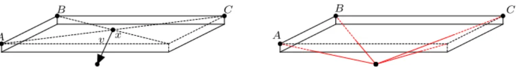
Note: as we don’t need the final value of the distance, it is only compared to determine the minimum, we don’t need to calculate the square root, only the expression inside the square root. However in 3D space it’s not so simple. We need the winner to pick the closest point to s, to pull this winner and its neighbours towards to s. Let P be a large flat cuboid (as it can be seen if Figure 1) , and letsbelow the cuboid. A central pointX on the other side is the closest point of the triangle’s corner forming the surface. If we select this as the winner, and pull it towards tos, the edges around X will cross the lower plane of the cuboid, and after the transformationP loses its spherical topology.
v x
B C
A A
B C
Figure 1: Selecting the winner from the wrong side
To prevent this behaviour, we must store the normal vectors of the triangles on the surface ofP. As we use the .OFF file format (mentioned early) to readP, and in this file the normal vectors are not stored – after reading and reconstruct- ing points and triangles ofP, we must calculate the normal vectors by ourselves.
To do this, we suppose that at the start phase P is convex. In this case if we havetriangle(A, B, C), we can calculate−*n normal vector by the following way(see Figure 2):
−−*
AB=B−A, −*
AC=C−A, −*n =−−* AB×−*
AC.
C
A
−* B AC
−−* AB
−
*v
Figure 2: A-B-C triangle and its normal vector
The−*n is a normal vector, but its direction might be wrong. The normal vector must point out of the body, not to its inner parts. We suppose that at this phase P is convex, so all the points ofP are on the same side of the plane defined by the triangle(A, B, C). In this case any of them can be a good representative (except the points, which lays on this plane as well). Select any pointxat the surface of P. Calculate−*
Axand its length. If it is not zero, thisxis suitable to determine the correct direction of−*n. If−*n points to the right direction, theαangle between−*n and −*
Axis a non-acute angle. Shift the two vectors to pointA, and calculate the value ofcosα:
−*
Ax:=x−A,k−* Axk:=p
(x.x−a.x)2+ (x.y−a.y)2+ (x.z−a.z)2
cosα:= −*n ·(x−A) k −*n kkx−Ak
Note: as we know, whenαis a non-acute angle,cosα <0. As we can see in the formula, the sign ofcosαdepends on the sign of the numerator, as the denominator always positive. So we need to evaluate the numerator expression only to determine the sign of cosα. If its sign is positive, we have to change the direction of −*n to point into the opposite direction.
At the beginning we suppose thatP has a spherical geometry, and we want to keep this property during the progress at all costs. According to this geometry, eachp∈P surface point can be a corner point of several edges (and so a part of several triangles). We will notate these asp.trianglesandp.edges.
Notice, than an edgeecan be attached to only two triangles at a time, according to the spherical topology of the object. When we examine any pointp from the surface, we must check all the p.triangles, their normal vectors to determine if the p point can be the winner or not. When all the normal vectors of all the p.trianglespoints away from s, then pcannot be selected as a winner. We must calculate the nominator of expression cosα again as (−*n +p)(s−p) for all the triangles containingp.
During the initial phase of the program, we load points P, reconstruct the triangles of the surface, and calculates all the normal vectors. It is important to keep the normal vectors, as later the P will lose its convexity, and we won’t be able to determine the correct direction of a−*n. When we update the coordinates of any of the points ofP, we must re-calculate of the normal vectors of the triangles based on this point. To do that, we can choose one of the following methods:
• At the beginning when the P was convex, and we determine the direction of the normal vector, we store the information that which was pointA, and after using −−*
AB and −*
AC to calculate the normal vector, we must switch its direction or not. With this extra information, we can recalculate the normal vector any time from now, after the changes of the coordinates.
• When any of the coordinates from A, B or C changes, we recalculate the normal vector immediately. The angle between the new normal vector and the old one must be a sharp angle (the coordinates change little), socosα≥0.
At GSOSM step 4 new points and new triangles are added to the surface – we must take care about their normal vectors as well. At GSOSM step 5 triangles disappears, and points moves heavily. This step will update the normal vectors of the remaining and affected triangles. We will talk about the calculating the normal vectors when we examine these steps closely.
At step 1 we select an s ∈ M randomly, then delete it from M to prevent selecting the sameslater. At step 3 we pull points towards tos, but as we will see later very slightly. After processing eachMpoints, thePwon’t be complex enough, and the surface ofP won’t fit tight. So we will process the points ofMseveral times again-and-again. The number of iteration is controlled by a parameter. When the repeat counter is set ton, we might imagine asM that it owns everys∈M points ntimes. As a set contains every element once, we might handleMas a list instead.
But in that case we might select s1 ∈ M, then s2 ∈ M to process, but it might happens thats1=s2, and the winnerwmoves towards to thesestwice in a short time. So we choose to store each point once in M, and construct an empty M0 set. Select ans∈M randomly, and delete it fromM, and add it toM0. WhenM becomes empty, we switch theM andM0, and continues the process with the full set again.
In [1] the points of P is organized into octree-based searching tree to speed up the searching process. Other possibility is to use the Point Cloud library itself, or the algorithm behind it. At the beginning of the implementation, we used a simple list to store the points. Inside this list, we use no special order, so to find the winnerw, we must check all the elements of the list.
4. GSOSM data structures
According to section 2, we use the following data structures for the GSOSM process:
1. Point3D(x,y,z)is a base data for storing a point’s coordinates in 3D space
2. Mesh(lp) holds a lists for the target body’s points on its surface given by coordinates,lpis “list of Point3D”
3. NVec(x,y,z) is a normal vector, wherex, y, zdefines the triangle of the plane 4. Triangle(e1,e2,e2,nv) is a triangle on a 3D object’s surface, given by three
edgese1,e2and e3, andnv stands for the normal vector of this triangle 5. Edge(a,b,lt) is an edge of a 3D object’s surface, where a and b are Points
(not Point3D, see later), and lt is a list of triangles based on this edge with exactly 2 elements on this list
6. Point(x,y,z,le,T) is an advanced point, which stores not only its coordinates, butlethe list of edges (and along with the edges the triangles as well) which are connected to this point, and T is the signal (active) counter, its value is 0 at the beginning (see 6)
7. Body(lp) is the body described by the list of Points (so the edges and the triangles are given as well).
We found, that in our un-optimized data structure step 1 and 2 (winner find and pulling) is about 34% of total time, the vertex split is about 6%, and the edge collapse is about 58% of total computation time.
5. GSOSM step 2: pulling w towards s
When we selects∈M to process, andw∈P as the winner, we pullw towardss along thep→svector. The percentage of the pulling defines the new position of w(marked asw0) in the following way:
−
*w0:= (1−λ)−*w+λ−*s .
This λvalue is the parameter of the algorithm. The more strong we pull, the faster theP fit tight toM. The more fast we pull, theP has less time to become complex enough, so the final shape ofP won’t be good enough.
Another problem appear as we test this part of the algorithm. If we pull strongly, the winner goes to s heavily. When we select another s0 ∈ M, close to the previous s, the same winner will be the closest again. In this case a peak arises from a flat space, and the shape of the part ofP cannot fit tight (see fig- ure 3). Later, we will see that the fact the samewwins again and again means it becomes highly active, and other points ofP turn into useless (inactive). We will erase them at step 5 using edge collapse, and we will lose a lot of points because the winner won’t let other points to win.
The other reason to keep λpercentage low is that the more complexP is, the more likely that after a pull ofw thew0 will arrive inside the body ofP (mainly whenP loses its convexity). With a small value ofλit is not 100% chance that it
Figure 3: The peak arises
won’t happen, but better chance to avoid this. Paper [1] advices the same, talks about unwanted effects, and chance to convergence to local minima or fold-overs.
The valueλis not a constant. At the beginning of the process, larger (but still small) values are better to let the P growing. Later we use smaller and smaller values. It is usual, that the value ofλis determined by a function, which argument is the progress percentage. This function converges to 0, to guarantee the conver- gence of the algorithm. Instead of a slowly calculable function we evaluate and fix these values in the parameters of the process, connecting the progress percentages with a constant value. When the progress percentage reaches the next limit, the λchanges its value to the next fix value. Paper [1] suggests using constant 6% for the whole process as an experimental value. The choice of this fraction is discussed in details in [4, 3].
5.1. Laplacian smoothing
After pulling the winner, [1] suggest using the Laplacian smoothing. In this case we select and move only the direct topological neighbours of the winner w. Let R(p) ={v1, v2, . . . , vn} be the direct topological neighbours of any p∈P. Let us calculate forvi ∈R(w)the LaplacianLas
L(vi) = 1 valence(vi)
X
vk∈R(vi)
(vk−vi).
When−*ni is one of the normal vectors of pointvi, the tangential component of Lcan be calculated as
Lt(vi) =L(vi)−(L(vi)· −*ni)−*ni
and we can update the coordinates ofvi tovi0 as vi0 =vi+αlLt(vi).
In this expressionαl is a constant parameter of the process, [1] suggests using αl= 0.06value, and suggest repeating this smoothing steps for 5 times.
5.2. Simple neighbours pulling
Another possibility is to update the direct or remote neighbours position is to use similar pulling towards tosas we used pullingw. We may use differentλvalues for pulling the neighbours as was used for pulling the winner, as we might use different λvalues for different distances from w. We might describe the pulling at a given percentage of the process with (p, λw, n, λ1, λ2, . . . , λn)tuple, where pdefines the process percentage,percwdescribes how strong must pull the winner,nstands for how far we must walk fromwwinner, andλi (i∈[1, n]) sets how strong we must pull theithneighbour towardss. This method was suggested originally in [3].
5.3. Elastic pull
This method is the “elastic pull” model. This provides a more flexible way to handle the pulling of the neighbours. In the elastic model the surface ofP can be imagined as the edges are made of a kind of material (soft rubber, hard and bold rubber, rubbed rope, or a stretchable metal). The material is described using a constant valueγ∈R, 05γ51. Larger value means more flexibility. So 0.0 (0%) means no stretch at all, while 1.0 (100%) means that the material can be stretched infinite.
When we have anedge(A, B)(a piece of rope), and we pull one end (A) of this edge towards a direction, we can calculate how much the edge become longer. For example after pulling endpoint A, the edge becomes 40% longer. When the rope is made from soft rubber, which has a valueλ, this rope can stretch easily, most of the energy of pulling is absorbed, the power is passed to the other end of the rope is only 0.4(1.0−0.8) = 0.08, which means 8%. This means, that the edges attached to endpointB stretches with 8% (pulling a point of a spider web causes other points of the web moving along with). The next edge will become longer with 8%, which causes the next level edge become longer with 0.08(1.0−0.8) = 0.016 (1.6%). As we can see, a rope with value 0.8 causes that each next edges will be less longer than the ones before. A rope with no ability to stretch (0.0) means that aM%stretching is passed to the next level withM%(1.0−0.0) =M%, so it forces the next level to stretch with the same amount. A value of 1.0 (100%, super elastic material) means no stretching force is passed,M%(1.0−1.0) = 0.0.
We can use different settings for different value of progression easily. At each progression percentage we can describe the elastic pulling as(p, f, min), where p is the percentage, f ∈ R, 0.0 5 f 5 1.0 the flexibility value of the edges, and min∈R, 0.05min < f is the minimal value of stretching.
6. Checking the topology of P
As we encounter several unwanted effects, we set up a method to check if any cross- pull happened withP. A cross-pull is when appoint goes inside the body, and any of thep.edges(a section) intersects any of the triangles of the surface. Lete(P, Q) an edge with the endpoints P and Q, and t(A, B, C) a triangle given by corner
Figure 4: Elastic pull a 2D sheet – without Laplacian smoothing
pointsA,B andC, and−*n is the normal vector of the triangle. We can check if an edgee intersects the plane determined by trianglet. We can use the equation for the plane determined by its’s normal vector and a point A of the plane:
n.x(x−A.x) +n.y(y−A.y) +n.z(z−A.z) = 0.
If we inserts both P and Qpoints into this equation, we can calculate the its final value. If one of the values is 0, that points rests in the plane, other values means the point is far from the plane. If the final values have different signs, it means the two points are in the different side of the plane, otherwise they are in the same side. So calculate the following final values:
p1=n.x(P.x−A.x) +n.y(P.y−A.y) +n.z(P.z−A.z) p2=n.x(Q.x−A.x) +n.y(Q.y−A.y) +n.z(Q.z−A.z).
Whenp1>0∧p2>0orp1<0∧p2<0the edgeedoes not intersect the plane of triangle t, so does not the intersect triangle t itself. If the previous condition evaluates to false: edgeeintersects the plane, but not necessarily intersects triangle t (maybe the intersection point is outside of the triangle). Another check must follow. First we calculate the intersection point coordinates (point q). We must need the direction vector of the line−*pq=Q−P, then we must use the parametric equation of a line S = P +t· −*pq : ∀t ∈ R produces point S on the lin. We are searching for that t∈Rwhich can be inserted into the equation of the plane and produces zero. So we must solve the equation:
n.x(P.x+t(Q.x−P.x)−A.x) +n.y(P.y+t(Q.y−P.y)−A.y)
+n.z(p.z+t(Q.z−P.z)−A.z) = 0.
After elementary steps we have:
t= n.x(P.x−A.x) +n.y(P.y−A.y) +n.z(P.z−A.z)
−(n.x·pq.x+n.y·pg.y+n.z·pq.z) .
We use insert this valuetback to the equation of the line, we give the intersection pointF as the following: F =A+t· −*pq.
Using this intersection point F we can check if it is outside the triangle t: if F.x5A.x∧F.x5B.x∧F.x5C.xorF.x=A.x∧F.x=B.x∧F.x=C.x(and the same happens withF.yandF.z) we can say that edgeewon’t intersect trianglet.
Otherwise, we calculate whether the point F and point A are on the same side of the line given by the two triangle points B-C. Using the same equations, we can write the equation of the line B-C based on point B as the following:
(x−B.x)(−C.y+B.y) + (y−B.y)(C.x−B.x) = 0. Inserting pointF andA into this equation, we can check if the values have the same signs or not, so are point F and A on the same side of the line. If for point F we got zero, it means the intersection point is on the line, which (in this case) means are on the same side.
Checking this for pointB(line based on pointsAandC), then for pointC(based on pointsAand B) we can check if the intersection point is inside the triangle or not. If it is inside, we have an error in the surface.
We must further check the spherical topology property ofP as well. It is done by:
• check that all the points p∈P have at least three edges
• all the edges must be associated exactly to two triangles.
7. Setting up “active” state
After selectingwwinner and pull towards tos, we increase the “active” counter of w with 1. Paper [1] says only the winner must be updated this way, we consider updating the selected neighbours as well. Otherwise, [1] says all the points of P (except for the winner) the value of this signal counter must be decreased by multiplying its value with α, where α∈R, 0 < α < 1. Paper [1] suggests using α= 0.95constant value.
This signal counter is used in section 9 to determine if a pointp∈P is active or not. When the value of the signal counter smaller than the required value, we delete pointpusingedge collapse.
Later this paper talks about the machine accuracy problem, and substitutes this method by a simple one: if a pointpwas not active since the last edge collapse – it must be handle as inactive point.
So we need only a logical value attached to each pointp, which are initially set tof alse. When a point is selected as a winner, we set this flag totrue. During the edge collapse phase, we handles all the points as inactive, which are stillf alse. At the end of the edge collapse, we set all remaining points back to f alse. Another way is when we have a global iteration counter, when apis selected to be a winner, we set the flag to the actual value of the counter (in which step was he selected winner). We can handle a point as inactive, when its “last winner flag” is too low, it has not been selected as a winner since the last edge collapse run.
8. Vertex split
As we described, steps 1–3 move the points of P towards the mesh M surface points. These steps will not increase (or decrease) the complexity ofP, so applying these steps won’t makeP to be very similar toM. Step 4 targets to makeP more complex by adding new points to it. Simply adding a new point won’t help, asP holds not only points but edges and triangles as well. After adding a new point we must insert it into the edges and triangles properly, keeping the spherical topology ofP.
First we select the environment where the new Qpoint can be added. Select the most activeA∈P point (with the highest signal counter value), and one of its direct topological neighbourB ∈P, the most active neighbours ofA.
Note: the standard method of vertex split suggests selecting point A∈P with the most valence, as this point really need splitting. If we have severalA1, . . . , An∈ P points with the same highest valence value, we can choose between them paying attention to its signal counter. An alternative way can be the following: select the A∈P to apply the vertex split finding the longest edge, or one of a triangle base point with the largest area.
Vertex split will happen using theedge(A, B)(there must be an edge betweenA andBas pointBis a direct topological neighbour of pointA). AsP has spherical topology, there must be exactly two triangles based on this edge, soAandB must have two common direct topological neighbours (C1 and C2). Let’s create a new pointC. This new point C won’t be on the section AB, as it is “edge split”, and we want to use “vertex split”. This new point C must be around A.
On a 2D space coordinates C might be chosen as an inner point either inside thetriangle(A, B, C1)or insidetriangle(A, B, C2).
A
B
C2 C1
r r
r
r r
r
r =⇒ A
B
C2 C1
r C r
r
r r
r . . . ...r
=⇒ A
B
C2 C1
r C r
r
r r
r r
Figure 5: Vertex split – first three phase
In 3D we can put this new point around the edge(A, B), not necessary on the triangles’ plane. Let’s calculate its coordinates as the following (for example):
C.x= (3/8A.x) + (3/8B.x) + (1/8C1.x) + (1/8C2.x) C.y= (3/8A.y) + (3/8B.y) + (1/8C1.y) + (1/8C2.y) C.z= (3/8A.z) + (3/8B.z) + (1/8C1.z) + (1/8C2.z).
The steps of vertex split are as follows:
1. add new pointCto the point list ofP with no edge and no triangle informa- tion
2. delete edge(A, B) and the triangles based on this edge (triangle(A, B, C1) andtriangle(A, B, C2)
3. create new edge(A, C) and edge(C, B) (don’t forget to add it to A.edges, B.edgesandC.edges)
4. create and insert triangle(A, C, C1), triangle(A, C, C2), thentriangle(C, B, C1)andtriangle(C, B, C2)into P properly.
Notice that at this point the valence ofAdoes not decreased, nor the complexity ofP increased, now we have 1 more edge, and 2 more triangles, and the long edge ABhas been replaced by two short edges.
A
B
C2 C1
C C3
C4 r r
r r
r r
r r r
r =⇒ A
B
C2 C1
C C3
C4 r r
r r
r r
r r r
r =⇒ A
B
C2 C1
C C3
C4 r r
r r
r r
r r r r
Figure 6: Vertex split – decreasing the valence ofA
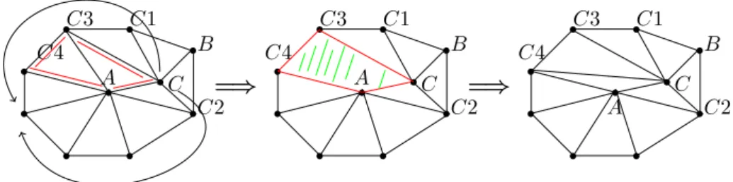
Further triangulation steps may be required. This time the steps are different (pis the selected point around A):
1. removeedge(A, p), so removetriangle(A, C, p)andtriangle(A, P, X)as well 2. define newedge(X, C)
3. define new trianglesX, C, P andX, A, C
4. only when the new edge does not intersects any faces except for the removed ones.
At this phase we added a new point C properly into the surface of P. This surface has no hole anymore, has more point than before (more complex). To do a better job at this point, we might want to redirect some edges of A into C, to decrease the valence of A, and increase of C. If A has a valence of n, we might want to redirectn/2 edges intoC.
To do that, first we gather all the direct neighbours points of A into setNA1. Notice: after execution of the previous steps, C, C1, C2∈NA1, butB is not. Let’s order these points as we could walk aroundA, starting fromC, going to the direc- tion towardsC1.
A
B
C2 C1
C C3
C4 r r
r r
r r
r r r
r =⇒ A
B
C2 C1
C C3
C4 r r
r r
r r
r r r
r =⇒
A
B
C2 C1
C C3
C4 r r
r r
r r
r r r r
Figure 7: Vertex splitted cube – without decreased valences
We might think it is a good idea to decrease the valence ofA, that processing this ordered list one-by-one we can redirect some edges toC. Select theA−C−C1−C3
quadrilateral, and follow the steps:
1. delete edge(A, C1)(decreasing the valence ofA), and all the triangles based on this edge (triangle(A, C, C1)andtriangle(A, C1, C3))
2. addedge(C, C3)(increasing the valence ofC) 3. addtriangle(C, C1, C3), and triangle(A, C, C3).
We can continue and repeat these steps walking around this direction for a few steps, and then we can turn around and walk on the other direction aroundA as well, redirecting the edges, untiln/2 edges are attached toC.
First of all: notice, that there is another possibility, than creating new edge (edge(C, C3)for example) between remote points: the edges can intersect the sur- face ofP. So after planning a redirect, we can check the integrity and correctness of the surface ofP using the method described in 6. If any error encounters, we step back to the correct state.
Second: what is working on 2D, won’t fit the 3D world. Let us suppose we have a cube, each square contains 2 triangles. One of the flats we vertex split, inserting a newC point and redirect the triangles on that square from the corner points to C. After this we find ourA−C−C1−C3quadrilateral, and follow the steps. On Figure 8 we can see the schematics and on Figure 9 we can see how a cube can be deformed by this method.
A C3
C1
C C
A C3
C2
Figure 8: Vertex splitted cube – before and after redirection
Figure 9: Vertex splitted cube after several steps
9. Edge collapse
According to the algorithm, we select s, find w, pull w towards s, somehow we pull the neighbours ofwtowardssas well, and sometimes we add new vertices to increase the complexity of P using vertex split. After a short time we will find, that P has inactive points, which never becomes a winner, they are far from the points ofM, and are useless. Then we can clear them by another standard method called edge collapse.
We can set when to execute this step based on the number of the vertices ofP (based on its complexity) or after everyν iterations. In [1] the suggested method is to execute after everyνniterations, whereν = 20, andnis the size ofP.
Selecting the less inactive or useless nodes we might select all the nodes which were not active (not selected as winner). We might expand the immunity against clearing to the ones which were selected and moved as a neighbour of any winner as well, however [1] suggests giving immunity only for the winners only.
When we select a nodea∈P to clear, we must select a direct neighbourb∈P as well. We will clear nodearedirecting its edges tob, sob’s valence will become higher.
First we know that this step seems to be very easy in 2D, but in 3D it can yield unwanted effects, and the spherical geometry can fail, but this effect arises at the end of the collapsing. So we advise to save the entire state ofP before the collapsing as it will be modified several ways, and we might roll back to the original state at the end. Another possibility is not to make any modification on the state of P, instead we collect the modification instructions into a list, then check the state of P according to this modifications steps, and if we find any failure, drop this list and do nothing.
In 2D the steps seems very easy and clear:
• delete edge(a, b), and all the triangles based on this edge (triangle(a, b, c) andtriangle(a, b, d))
• find every triangles containing point a, and replace this corner point to b (there is no triangle still exists which contains not only a and b as well, because we drop them at the previous step)
• delete pointa, as it loses any connection to other points on the surface ofP.
c
d
a b
Figure 10: Edge collapse
The main problem is in step 2. When we have atriangle(x, y, a)for example, we must replaceedge(x, a)toedge(x, b). Might there is already anedge(x, b)inP, so this step sometimes creates a new edge, sometimes not. The same is true for the triangles: triangle(x, y, a) becomes triangle(x, y, b), but sometimes this triangle already exists.
To demonstrate the problem, see figure 11. We have a tetrahedronA−B−C−D with point E on the edge between BD. It is interesting, that collapsing B →E won’t cause any problem, we would drop triangles A−E−B and E−B−C, and triangleA−B−Cwould become A−E−C which will close the shape, and the tetrahedron still remain tetrahedron. But if we try to collapse edge E → A, the whole side covered withA−B−E andA−E−B triangles would disappear.
After thatB−E−C goes intoB−A−C which is already exists, andE−C−B changes toA−C−Bwhich already exists as well. After the edge collapse steps we would have only two triangles, and the shape of this 3D object loses its spherical geometry and becomes a folded paper. This is the reason why we must prepare to roll back the edge collapse at any step we made.
A
C D
B
A
B C D
Figure 11: Edge collapse fails
Acknowledgements. First we want to thank to Annamária Stefán, who helped to develop and test the application, and gives several tips related to the topic. Besides, we want to thank László Balog who developed the useful tool, theTurnOffTheWorld application, which shows us the results of the GSOSM processing. Least but not
last we want to thank Miklós Hoffmann for supportive presence in this project, for his guidance, for his patience, and the constant pleasant atmosphere he created.
References
[1] I. P. Ivrissimitzis, W-K. Jeong, H-P. Seidel, Using Growing Cell Structures for Surface Reconstruction, Shape Modeling International, 2003, ISBN: 0-7695-1909-1, Page 78–86, 12–15 May 2003.
[2] The Point Cloud library (http://www.pointclouds.org).
[3] Hoffmann M., Numerical control of Kohonen neural network for scattered data approximation, Numerical Algorithms 39, 175–186, 2005.
[4] Hoffmann, M., Modified Kohonen Neural Network for Surface Reconstruction, Publ. Math., 54 suppl., 857–764., 1999.
[5] Tobor, I., Reuter, P., Schlick, C., Multi-scale reconstruction of implicit sur- faces with attributes from large unorganized point sets, Shape Modeling Applications, 2004. Proceedings, pp. 19–30, 2004.
[6] Yutaka Ohtake, Alexander Belyaev, Hans-Peter Seidel, Sparse Surface Re- construction with Adaptive Partition of Unity and Radial Basis Functions, Graphical Models, 68(1), pp. 15–24, 2006.
[7] Qi Xia, Shatin Wang, Xiaojun Wu, Orthogonal Least Squares in Partition of Unity Surface Reconstruction with Radial Basis Function, Geometric Modeling and Imaging–New Trends, 2006, pp. 28–33.
[8] Yi-Ling Chen, Shang-Hong Lai, A Partition-of-Unity Based Algorithm for Im- plicit Surface Reconstruction Using Belief Propagation, In Proceedings of Shape Modeling International 2007 (SMI’07), Lyon, France, June 2007.
[9] B. Fritzke, Growing Cell Structures – a self-organizing network for unsupervised and supervised learning, Neural Networks vol 7. no. 9, pp. 1441–1460, 1994.
[10] B. Fritzke, A growing neural gas network learns topologies, Advances in Neural Information Processing Systems, vol 7, MIT Press, pp. 625–632, 1995.
[11] Ivrissimtzis, Ioannis, Jeong, Won-Ki, Seidel, Hans-Peter, Neural meshes:
statistical learning methods in surface reconstruction, Max-Planck-Institut für Infor- matik, MPI-I-2003-4-007, ISSN: 0946-011X, 2003.
[12] Vilson Luiz Dalle Mole, Aluizio Fausto Ribeiro Araújo, Growing Self- Organizing Surface Map: Learning a Surface Topology from a Point Cloud, Neural Computation Vol. 22, No. 3, pp. 689–729, 2010.
[13] http://people.sc.fsu.edu/~jburkardt/data/off/off.html